Troubleshooting & Monitoring Queries

Deephaven provides a number of options to enable users to monitor query performance and resolve issues as they arise. Many of these methods are available directly in the user interface. For example, users can see how long a query has been running by opening the History Panel and looking at the command details, or by hovering over the command in the console: the tooltip will show the formatted duration of the query. The most common performance issues are slow initialization, a query failing to update quickly, or a sluggish user interface.

This chapter first discusses where to find performance information and how to interpret it. If a query seems to be taking too long or throws an error, users may look to Deephaven's Internal Tables, which contain general performance details about Deephaven processes and workers. These tables can be queried individually to diagnose slow or unresponsive queries. Several of these internal tables can be opened at one time with the performanceOverview() method, which is particularly helpful when investigating reasons when a query is not responding as expected. After describing each of the tables called up by the performanceOverview() method, this chapter then offers a number of solutions and best practices to ensure your queries run smoothly.

While these techniques are intended to help you troubleshoot queries independently, Deephaven Support is always just a click away. When serious or unexpected errors arise, we recommend you send your Console logs and/or Exception messages.

Internal Tables

All Deephaven installations include several tables that contain specific information for the system's internal use. These internal tables are updated by various processes, and contain details about processes and workers, and the state of persistent queries and all query operations. These tables are stored in the DbInternal namespace.

Just like other tables, authorized users can run queries against these internal tables. The following provides an in-depth look at the most important tables when it comes to troubleshooting queries, and what to look for in these log reports:

• QueryOperationPerformanceLog
• UpdatePerformanceLog
• PersistentQueryStateLog
• ProcessEventLog

QueryOperationPerformanceLog and UpdatePerformanceLog

The QueryOperationPerformanceLog provides information about performance details on Deephaven query operations, such as duration and memory usage. To view this table, run the following query:

QOPL = db.i("DbInternal", "QueryOperationPerformanceLog")\
    .where("Date=currentDateNy()")

Each query is broken up into its component parts, allowing a comprehensive understanding of the performance impacts of each individual operation for a query. Columns include (among others):

• ServerHost
• ClientHost
• WorkerName
• Description
• StartTime
• EndTime
• Duration
• TotalMemoryChange
• WasInterrupted

If a query is not updating as quickly as expected, or the UI seems slow, you can view the UpdatePerformanceLog for information about incremental update operations:

UPL=db.i("DbInternal", "UpdatePerformanceLog")\
    .where("Date=currentDateNy()")

Columns include (among others):

• ServerHost
• WorkerName
• WorkerStartTime
• ClientHost
• QueryName
• EntryDescription
• IntervalStartTime
• IntervalEndTime
• IntervalDuration
• EntryIntervalUsage
• TotalMemoryUsed

The "Description" or "EntryDescription" column includes human-readable information that describes the type of operation. Below is a snippet of the Description column from the QueryOperationPerformanceLog, where you can see logs related persistent queries that open the StockTrades and StockQuotes tables from the LearnDeephaven namespace. (Note that the columns referenced in this explanation have been moved to the front of the QueryOperationPerformanceLog.)

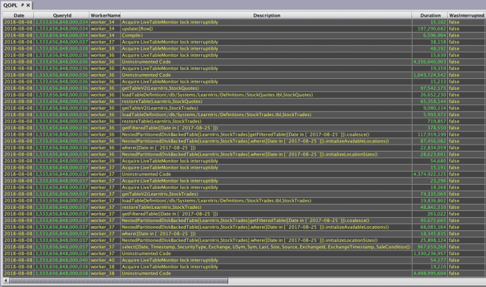
The majority of the entries in this column indicate each operation performed on a table (e.g., join, sort, where, etc.). Looking at other columns in a given row, such as Duration or WasInterrupted, may help you determine which specific operations are slow and, subsequently, offer hints as to how to resolve the issue. Details follow about other common entries in these logs. None of these log descriptions are cause for concern on their own. However, in general, any action that takes a long time could be contributing to performance issues.

• Acquire LiveTableMonitor lock or Acquire LiveTableMonitor lock interruptibly — These can help users to discern when LTM lock contention is the cause of query slowness or unresponsiveness. In the latter case, another thread can potentially interrupt the LTM cycle, affecting how frequently data is updated on the server. To learn more, see Live Table Monitor.
• Aggregated Small Updates (UpdatePerformanceLog only) — A summary description that indicates a group of updates, where each of which is less than the configurable threshold for logging an update. For many workloads, the vast majority of updates will not materially affect performance. By aggregating the updates, significant disk space and bandwidth may be saved. The threshold for update logging may be configured with the QueryPerformance.minimumUpdateLogDurationNanos, QueryPerformance.minimumUpdateLogRepeatedDataReads, and QueryPerformance.minimumUpdateLogFirstTimeDataReads properties. See Filtering Small QueryOperationPerformanceLog and UpdatePerformanceLog Entries below.
• compile — Calls to the Java compiler to translate Deephaven query language expressions into JVM bytecode (classes). If your workload has excessive compilation time, you may consider reusing formulas and providing parameters through the QueryScope. See Steps for Reducing Ratio.
• coalesce() — Describes producing a QueryTable that can be used for query operations from an UncoalescedTable (typically a SourceTable). The SourceTable is a placeholder that represents your data and defers most work until a query operation is required, at which point it must be coalesced.
• .initializeAvailableLocations() and .initializeLocationSizes() — These actions require filesystem access to read directories (locations) and then many table.size files. This can have a substantial impact on a historical query.
• Uninstrumented Code — This is code that is not enclosed in a measurement block, which means it cannot be monitored or traced. It could indicate a bug, or a complex operation that, because it is outside of our framework, has no details available.

Filtering Small QueryOperationPerformanceLog and UpdatePerformanceLog Entries

The UpdatePerformanceLog is extremely comprehensive, and contains many small entries (Aggregated Small Updates) that are not always of interest for debugging performance. Users can set a minimum threshold to filter out these small entries, which frees up disk space and makes it easier to analyze the tables.

Three properties configure minimum thresholds for the UpdatePerformanceLog (minimumUpdateLog), three properties configure minimum thresholds for the QueryOpertationPerformanceLog (minimumLog), and three properties configure minimum thresholds for uninstrumented code (minimumUninstrumentedLog):

• QueryPerformance.minimumUpdateLogDurationNanos=<nanoseconds> — sets a minimum duration in nanoseconds for recorded entries in the UpdatePerformanceLog. For example, setting this property to =1000000 discards entries in the UpdatePerformanceLog with a duration less than a millisecond. When set to 0, all values are logged.
• QueryPerformance.minimumUpdateLogRepeatedDataReads — sets a minimum threshold of repeated data reads (reading a block of data from another service or the disk) to be recorded in the UpdatePerformanceLog. For example, when set to =1, only one repeated data read will be recorded. This value may not be 0. If set to a negative value, then update performance for repeated or first-time data reads will not be logged.
• QueryPerformance.minimumUpdateLogFirstTimeDataReads — sets a minimum threshold of first-time data reads to be recorded in the UpdatePerformanceLog. This value may not be 0. If set to a negative value, then update performance for repeated or first-time data reads will not be logged.
• QueryPerformance.minimumLogDurationNanos — sets a minimum duration in nanoseconds for recorded entries in the QueryOperationsPerformanceLog. When set to 0, all values are logged.
• QueryPerformance.minimumLogRepeatedDataReads — sets a minimum threshold of repeated data reads to be recorded in the QueryOperationsPerformanceLog. This value may not be 0. If set to a negative value, then update performance for repeated or first-time data reads will not be logged.
• QueryPerformance.minimumLogFirstTimeDataReads — sets a minimum threshold of first-time data reads to be recorded in the QueryOperationsPerformanceLog. This value may not be 0. If set to a negative value, then update performance for repeated or first-time data reads will not be logged.
• QueryPerformance.minimumUninstrumentedLogDurationNanos — sets a minimum duration in nanoseconds of uninstrumented code to be recorded in the QueryOperationsPerformanceLog. When set to 0, all values are logged.
• QueryPerformance.minimumUninstrumentedLogRepeatedDataReads — sets a minimum threshold of uninstrumented repeated data reads to be recorded in the QueryOperationsPerformanceLog. This value may not be 0. If set to a negative value, then update performance for repeated or first-time data reads will not be logged.
• QueryPerformance.minimumUninstrumentedLogFirstTimeDataReads — sets a minimum threshold of uninstrumented first-time data reads to be recorded in the QueryOperationsPerformanceLog. This value may not be 0. If set to a negative value, then update performance for repeated or first-time data reads will not be logged.

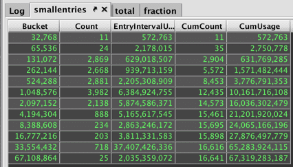
To determine how many small entries actually exist in your system, run the following query to create three tables with specific totals and usage information:

smallentries=db.i("DbInternal", "UpdatePerformanceLog")\
    .where("Date=currentDateNy()")\
    .updateView("Bucket=Long.highestOneBit(EntryIntervalUsage)")\
    .view("Count=1", "Bucket", "EntryIntervalUsage")\
    .sumBy("Bucket").sort("Bucket")\
    .by()\
    .updateView("CumCount=cumsum(Count)", "CumUsage=cumsum(EntryIntervalUsage)")\
    .ungroup()
total=smallentries.view("Total=Count", "TotalUsage=EntryIntervalUsage")\
    .sumBy()
fraction=smallentries.naturalJoin(total, "")\
    .updateView("FracEntries=CumCount/Total", "FracTime=CumUsage/TotalUsage")

The "smallentries" table sources its data from the UpdatePerformanceLog for the current date.

• The first .updateView operation creates a column named Bucket that rounds up the EntryIntervalUsage value to the next highest power of two.
• The .sumBy method sums the Count column, defined as 1, and the actual EntryIntervalUsage value, and then sorts the first entries into the lowest bucket.
• The .by method converts the table into one row with the content placed into arrays.
• The second .updateView operation creates the CumCount and CumUsage columns: these will display the cumulative counts/cumulative usages by bucket.
• Finally, the .ungroup() method places the content back into a multi-row table.

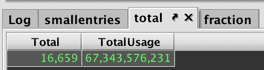
The "total" table shows a ticking total of the number of entries and their usage:

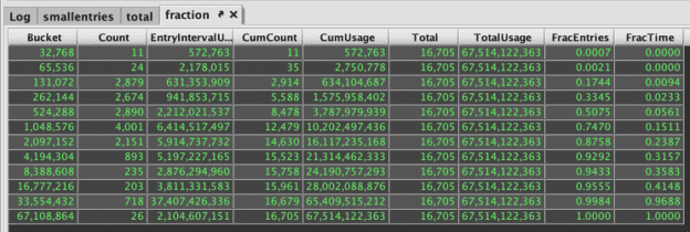
The fraction table contains the fraction of entries and time for each bucket of usage:

PersistentQueryStateLog

Persistent query processes record their activity and state in the PersistentQueryStateLog table, which can be used to see both the current state of any persistent query as well as all the historical states. To view this table, run the following query:

PQSL=db.i("DbInternal", "PersistentQueryStateLog")\
    .where("Date=currentDateNy()")

When errors or exceptions occur, refer to this table to pinpoint queries that have failed and to view the error messages.

The "Status" column in the PersistentQueryStateLog shows current state of all queries, such as:

• Connected
• Acquiring Worker
• Initializing
• Completed
• Running
• Stopped
• Failed

The status of failed queries could be failed, error, or disconnected.

Failed

This means that the persistent query failed before or during initialization. Refer to the ExceptionMessage column in the PersistentQueryStateLog for specific details.

• The most common cause of failure is an error in the script. When you hover over a cell, the tooltip displays the full text of the error message, which will pinpoint the first location where an error is encountered. For instance, if you leave out a closing quotation mark around a string, you will see java.lang.RuntimeException, the line number of the error, and a suggestion to correct it: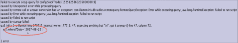
• A query may also fail to initialize because starting a new query exceeds the query server's maximum heap size. If you suspect this is the case, first try increasing the memory (heap) usage value in the Persistent Query Configuration Editor.

Error

This means that an error occurred after the query was initialized (e.g., while processing incremental updates). The ExceptionStackTrace column may offer more information in this case. To review this information, hover your cursor over the cell, or right-click the entry and select Show Value to open a dialog window with the full text.

Disconnected

The worker process disconnected from the dispatcher. The RemoteQueryProcessor (query worker) disconnects from the RemoteQueryDispatcher typically as a result of an exceptional error, or too much workload that prevents the worker from sending a heartbeat. Common reasons for a disconnection include:

• The server runs out of heap and an OutOfMemoryError notification occurs, thus killing the JVM.
• The JVM is stuck in Garbage Collection so long that it is unable to respond to dispatcher heartbeats for 60 seconds.
• A deployment issue results in a NoSuchMethodError. -An error occurred in internal JVM or a native code error occurred (aka, a JVM Hotspot Error).

Running the following query will show all the times a persistent query entered a failure state on the current date:

pqsAllFailedStates = db.i("DbInternal","PersistentQueryStateLog")\
    .where("Date=currentDateNy()", "Status in `Failed`, `Error`, `Disconnected`")

Adding a lastBy() call to the query shows the most recent state of any persistent query that attempted to start on the current date:

pqslAllCurrentStates = db.i("DbInternal","PersistentQueryStateLog")\
    .where("Date=currentDateNy()").lastBy("SerialNumber")

Combining the above queries indicates which persistent queries are currently in a failure state:

pqslCurrentFailedStates = db.i("DbInternal","PersistentQueryStateLog")\
    .where("Date=currentDateNy()")\
    .lastBy("SerialNumber")\
    .where("Status in `Failed`, `Error`, `Disconnected`")

Alternatively, the Query Config panel in the Deephaven Console also provides details about the persistent queries that you are authorized to see. Information about each query is stored in columns, including the owner, the query name, whether it's enabled, and its status. If a persistent query has failed, the column titled "Exception Details" (which includes the same raw data as the PersistentQueryStateLog) may contain content pertinent to why the query failed.

To read the Exception Details, hover the mouse pointer over the cell. This will open a tooltip window that displays the full content.

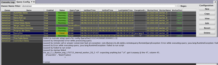
In the example above, "QueryOne" has failed due to a script error (java.lang.RuntimeException). Just as in the PersistentQueryStateLog, the tooltip suggests a solution to revise the script. In this case, the closing quotation mark is missing after the table name, StockTrades.

However, this option only allows the review of this content while the tooltip is activated. For other options, right-click on the cell containing the Exception Details for your specific query.

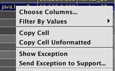
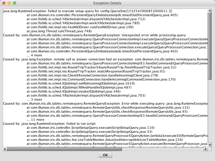
To view the Exception Details in their own window, select Show Exception in the drop-down menu.

To open a support ticket, select Send Exception to Support.... This will open a dialog window similar to the one shown below:

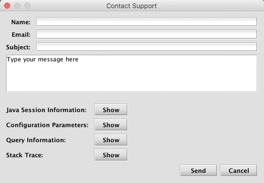
You should first enter your name and email address in the respective fields. A descriptive subject line should be included in the Subject field, and sufficient details about the issue should be included in the Message field.

The Java Session Information, Configuration Parameters, Query Information, and Stack Trace will automatically be attached to the email when sent. You can review the information contained in each by clicking the respective Show button.

ProcessEventLog

The ProcessEventLog contains log messages from Deephaven processes, and enables users to see logs from their own worker without server access.

To find all FATAL Level messages in the ProcessEventLog, the following query can be used:

t = db.i("DbInternal","ProcessEventLog")\
    .where("Date=currentDateNy()", "Level=`FATAL`")

To find error messages for a specific query worker, you can locate worker name and worker host in the Query Config panel or the Deephaven Console, and use these values to query the ProcessEventLog:

t = db.i("DbInternal","ProcessEventLog")\
    .where("Date=currentDateNy()")\
    .where("Host=workerHost")\
    .where("Process=worker_name")\
    .where("LogEntry.contains(errorText)")

Hover over the cell for your query in the "Log Entry" column to view the full exception message and stack trace from the results of the query, or right-click on the cell and select Show Value to open the text in its own dialog window.

The ProcessEventLog can also help users determine when query slowness or unresponsiveness is caused by other requests that have consumed all available threads in the serial or concurrent request thread pools in the LiveTableMonitor cycle.

The following log lines are observable in the ProcessEventLog or text-based worker logs:

<description>: running after <delay> ms waiting

While users can query the internal tables directly, the performanceOverview method opens a set of performance tables at one time.

Performance Overview

Typing performanceOverview() into the console provides simple and immediate access to performance logs and tables sorted in various ways, such as to show the operations taking the longest.

The following methods are available:

• performanceOverview() opens performance data about the current worker.
• performanceOverview(workerNumber) displays performance data for a specified worker, where workerNumber is the worker indicated in the console window, or in the Query Config panel. Calling the method from one worker to monitor another prevents the processing required by the performanceOverview() method from affecting the resultant performance data.
• performanceOverview(18, "2018-06-21") opens performance data for a particular date. In addition to any String date, you can use lastBusinessDateNy() or currentDateNy().
• performanceOverview(18, lastBusinessDateNy(), true) opens performance data for worker_18 on the last business date. Including true will cause the DB to look at the performance logs with db.i() instead of db.t(). This is useful when historical data merges for DbInternal have not been configured.
• performanceOverview(18, lastBusinessDateNy(), true, "0.0.0.0") is the same as the previous example, but adds a filter to specify the IP address of the server host (0.0.0.0 in this case). This can help disambiguate when one worker is serving requests originating from several different servers.
• performanceOverview("workerName" = null, "`YYYY-DD-MM`"= null, useIntraday = true, serverHost = db.getServerHost(), "workerHostName"=null) includes an additional workerHostName parameter, which may be required if the specified workerName exists on multiple query servers for the given date. In the case that multiple queryServers have executed the worker, then the "Host" column of the LTMCycles will identify multiple hosts, and the resultant charts will be non-linear. The appropriate workerHostName should be determined from this list of hosts; this may be an IP or an alternative alias to the host.
• performanceOverviewByName("queryName", "queryOwner") will produce the exact same performance data as performanceOverview(), but will instead filter to data related to the query named, "queryName", which is owned by the query author, "queryOwner".
• performanceOverviewByName("queryName", "queryOwner", "`YYYY-DD-MM`"= null, useIntraday=true, DBDateTime asOfTime = DBTimeUtils.currentTime())includes an additional asOfTime parameter, which will let you differentiate potential different restarts of a worker.

The performanceOverview commands opens several tables and, if applicable, one widget:

1. queryPerformanceLog
2. QueriesMostRecent
3. queryOps
4. QueryOpsLongest
5. QueryOpsMostRecent
6. maxHeap
7. updatePerformanceLog
8. UpdateWorst
9. UpdateMostRecent
10. UpdateAggregate
11. UpdateSummaryStats
12. WorkerLogs
13. gcLogs
14. gcPerSec
15. parNewLogs
16. LivenessCount
17. LTM Cycles
18. LTMBins1Minute
19. LTMCycleTimeline (plot)
20. PerformanceTimeline (plot)

The QueryOpsLongest table explicitly shows you the longest steps of your query's initialization process. For queries using intraday data, initialization is only part of the picture. The QueryOpsLongest table shows the longest parts of query initialization, but queries using live data also have to update results after initialization, as new data flows in. If you have an intraday query that has trouble keeping up with real-time data, you should look at the UpdateWorst table.

In UpdateWorst, the column to focus on is Ratio. The Ratio value shows what percentage of a query's data refresh cycle is consumed by each operation. If the sum of the Ratio column for one update interval approaches 1.00 (100%), then the query will be unable to keep up with incoming data. When you configure Deephaven for multi-threaded update processing (LiveTableMonitor.updateThreads=N), your ratio may exceed 1.0. In this case, the ratio can approach N * 1.00, where N is the number of threads. As using threads for updates respects dependencies, analysis may be more difficult, as the system might not be able to reach the total ratio of N due to unsatisfied dependencies or long chains of serial operations. You should also carefully monitor the IntervalDuration to ensure it does not exceed 61 seconds. The sum of the Ratio column for each interval, as a percentage, is available in the UpdateAggregate table. See Steps for Reducing Ratio.

Below is a full description of each table that performanceOverview() produces, broken up by category.

Query Initialization

queryPerformanceLog

This table contains top-level performance information for each query executed by the given worker. It contains data on how long each query takes to run.

A query, in this context, is the code that is run:

• Whenever you type a new command in the console and type Return. Each 'return' where you have to wait for an answer from the query server is a new query.
• When a persistent query initializes.
• When a Java application calls RemoteQueryClient.sendQuery() or RemoteQueryClient.sendNewQuery().
• As a result of a sort, filter or custom column generated in the GUI.

The most significant columns in this table are:

• TimeSecs — How long this query ran for, in seconds.
• TotalSecsFirstReads — Total time spent reading data into memory (and cache) for the first time.
• TotalSecsRepeatReads — Total time spent re-reading data (repeat reads are when we have a subsequent cache miss and need to reread a block that we know has been previously read).
• QueryMemUsed — Memory in use by the query (only includes active heap memory).
• QueryMemUsedPct — Memory usage as a percentage of the max heap size (-Xmx).
• QueryMemFree — Remaining memory until the query runs into the max heap size.

QueriesMostRecent

This table sorts the queryPerformanceLog to show the most recently completed query operations.

queryOps

This table contains performance information for each operation run by a query. Every call to the standard table operations [select(), update(), view(), updateView(), sumBy(), avgBy(), etc.] constitutes a distinct operation.

The most significant columns in this table are:

• StartTime — The time at which this operation started.
• EndTime — The time at which this operation ended.
• OperationNumber — Monotonically increasing sequence numbers for each operation of a query.
• TimeSecs — The time (in seconds) that the operation took.
• NetMemoryChange — The change in memory usage while this operation was occurring. Memory usage is affected by factors beside the currently running operation; as a result, NetMemoryChange is only an approximation of the memory impact of each operation. NetMemoryChange = TotalMemoryChange - FreeMemoryChange, where "total memory" is memory reserved by the JVM for heap, and "free memory" is how much has not been used yet. The NetMemoryChange value will be negative when memory allocation is high, and its value will be positive when there is a large amount of GC. Sorting on NetMemoryChange should provide a useful overview of which operations are taking the most memory.
• QueryMemoryUsed — The total amount of memory used by the worker.
• QueryMemUsedPct — Memory usage as a percentage of the max heap size (-Xmx).
• QueryMemoryFree — The total amount of free memory remaining. This is the difference of WorkerHeapSize and QueryMemoryUsed. If this approaches zero, a query is likely to experience poor performance or crash due to an OutOfMemoryError.
• WorkerHeapSize — The maximum heap size for the query worker.
• TotalSecsFirstReads — Total time spent reading data into memory (and cache) for the first time.
• TotalSecsRepeatReads — Total time spent re-reading data (repeat reads are when we have a subsequent cache miss and need to reread a block that we know has been previously read).

QueryOpsLongest

This the queryOps table sorted to show the most time-consuming operations at the top of the table.

QueryOpsMostRecent

This the queryOps table sorted to show the most recently completed query operations at the top of the table.

Real-Time Updates

For queries operating on ticking data (e.g., intraday data or Input Tables), there are additional logs detailing the time consumed updating tables with the new data.

maxHeap

This table finds the query's maximum heap size.

updatePerformanceLog

This table describes what the query spent time on during its data refresh cycle. This data is written in predefined intervals; the default is one minute, but it can be configured per query. At the end of each performance monitoring interval, a query logs every operation whose results were updated, and how much time it spent performing that update throughout the interval.

The most significant columns are:

• IntervalStartTime — The start time of the interval.
• IntervalEndTime — The end time of the interval.
• IntervalDuration — The duration of the performance monitoring interval, in nanoseconds.
• Ratio — This is the percentage of the performance monitoring interval that was consumed updating each operation. This is an approximation of how much of the available CPU was used by a given operation.
• QueryMemoryUsed — The total amount of memory used by the worker.
• QueryMemUsedPct — Memory usage as a percentage of the max heap size (-Xmx).
• QueryMemoryFree — The total amount of free memory remaining. This is the difference of WorkerHeapSize and QueryMemoryUsed. If this approaches zero, a query is likely to experience poor performance or crash due to an OutOfMemoryError.
• WorkerHeapSize — The maximum heap size for the query worker.
• TotalMemoryFree — Total free memory within the worker relative to the allocated heap size (not the maximum heap size).
• TotalMemoryUsed — Total memory used by the worker. The JVM will automatically increase this as necessary, until it reaches the worker's configured max heap size.
• NRows — Total number of changed rows.
• RowsPerSec — Average rate data is ticking at.
• RowsPerCPUSec — Approximation of how fast CPU handles row changes.

UpdateWorst

This table is the updatePerformanceLog sorted to show the slowest-updating operations, out of all intervals since the query initialized, at the beginning of the table ( i.e., the operations with the greatest "Ratio").

UpdateMostRecent

This table is the updatePerformanceLog sorted to show the most recent updates first. Operations are still sorted with the greatest "Ratio" at the beginning of the table.

UpdateAggregate

This table shows update performance data aggregated for each performance recording interval. The "Ratio" in this table represents the total CPU usage of each individual operation displayed in the other tables. If the "Ratio" in this table regularly approaches 100%, it indicates that the query may be unable to process all data updates within the target cycle time (the set target time for one LTM cycle to complete). This can result in delayed data updates in the UI.

UpdateSummaryStats

This table takes the data in UpdateAggregate and aggregates it into a single row view of the 99th, 90th, 75th, and 50th percentiles of "Ratio" and "QueryMemUsedPct" over all intervals, which makes the spread of resource consumption easier to view.

Other Tables

WorkerLogs

This table is the ProcessEventLog for the specified worker.

gcLogs

This table aims to show every time garbage collection (or "GC") runs, for queries with GC logging enabled. Garbage collection is a memory management process that automatically collects unused objects created on the heap and deletes them to free up memory. The JVM's GC logs contain information about how often GC is performed and other details of the collection process. Examining these logs helps determine if queries do not have enough memory. More information about GC log patterns can be found in Deephaven Operations Guide.

gcLogsPerSec

This table shows how long GC takes.

parNewLogs

This table attempts to parse time spent on ParNews out of the GC logs. ParNew GC is a stop-the-world, copying collector which uses multiple GC threads (a parallel collector algorithm). See GC Log Patterns.

LivenessCount

The LivenessCount table records the outstanding referent count for that worker, as well as the smallest number (the intervalMin column) and largest number (the intervalMax column) since the last time they were logged. In the example for worker_110 below, we see that the count begins at 0, then jumps to 16, within the 20s, and finally hovers around 30:

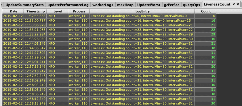
When a query executes (such as a tree table opening), the count increases, and objects are created for operations such creating empty tables and timetables, performing selection methods, sorts, filters, etc. Each one of these processes makes listeners, sub-tables and related artifacts that are included in the referent count. Deephaven's built-in Liveness instrumentation releases any objects created in the GUI that are no longer needed or are not refreshing. Here, the count moves between 31 and 30 as an object is let go. Closing the tables will bring the reference count down towards 0.

A high referent count/liveness count is not a concern in and of itself. A complex query may require many objects; however, the count should consistently go back down to a baseline number.

LTMCycles

This table will show the length of LTM cycles. The LiveTableMonitor (or "LTM") is the part of the query engine that handles real-time data updates. It runs in cycles (once per second, by default). When LTM cycle logging is enabled, the LTM will write the cycle's length to the logs (e.g. "Live Table Monitor Cycle Time: 472ms") every time it completes a cycle.

LTMBins1Minute

The columns in this table display information about Live Table Monitor cycles that finished during each timebin. Deephaven tables only update to reflect new data when a LTM cycle completes. These statistics can help assess queries that appear to update infrequently or not at all. In general, it is preferred that LTM cycle times do not exceed 1 second (i.e., 1,000 ms, in the LTMBins1Minute table). Note that there will be no LTM cycles when there are no source data changes.

The columns in this table are:

• Min - The shortest LTM cycle that completed during a one-minute period.
• P50 - The median (50th percentile) duration of LTM cycles that completed during a one-minute period.
• P95 - The 95th percentile of LTM cycles durations that completed during one one-minute period.
• P99 - The 99th percentile of LTM cycles durations that completed during one one-minute period.
• Max - The longest LTM cycle that completed during a one-minute period.
• Avg - The average duration of LTM cycles that completed during a one-minute period.
• Count - The number of LTM cycles that finished in a one-minute period.

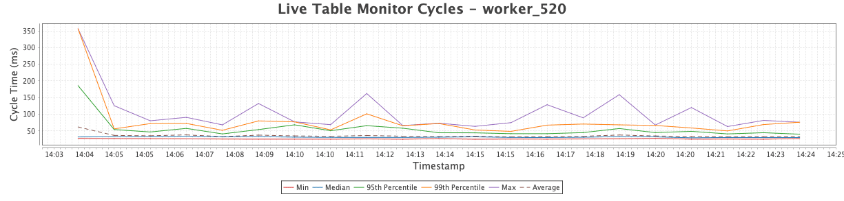
LTMCycleTimeline

The LTMCycleTimeline widget plots LTM cycle time values from the LTMBins1Minute table:

PerformanceTimeline

The PerformanceTimeline widget will appear only if there is data in either the UpdateAggregate table or the LTMCycles table at the time that performanceOverview() is run.

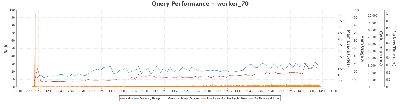
Ratio values appear along the Y axis: ParNew Real Time (in seconds), Cycle Length (in milliseconds), Memory Usage (in percentage), and Memory Usage (in bytes). The data from the LivenessCount table is also plotted. For example, the close-up of the PerformanceTimeline below shows the values for worker_110 shown above. The LivenessCount graph consistently returns to approximately the count of 30:

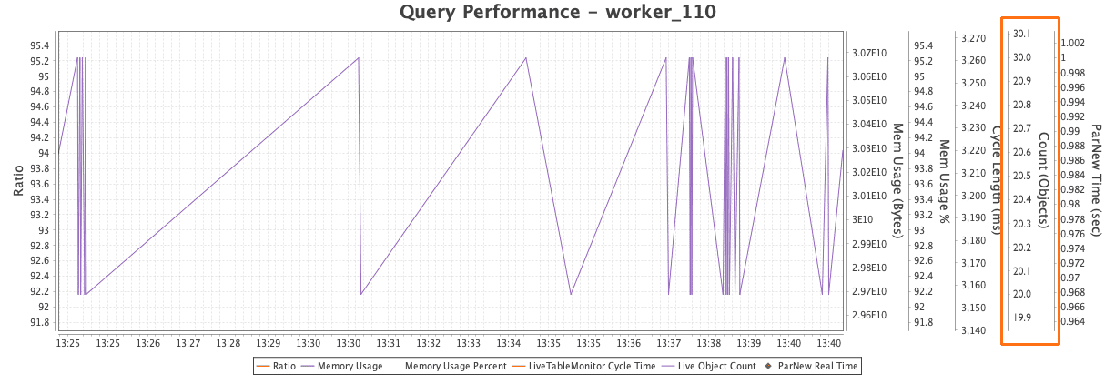
A simple query on static tables that does not create new objects would produce a flat line. So, a particularly steep line might suggest that objects are not being properly tracked and released. In this case, the values frequently move around spike upwards, but always go back down to the same point.

Persistent Query Status Monitor

Typing persistentQueryStatusMonitor() into a console will gather and aggregate performance data pertaining to your persistent queries and join them onto the Persistent Query State Log. This enables you to see if your queries are running and provides various metrics related to their performance.

The following methods are available:

• persistentQueryStatusMonitor() opens several tables related to the performance of your persistent queries on the current date.
• persistentQueryStatusMonitor("startDate", "endDate") opens performance data for a particular period of time. This allows you to include previous dates as you may be interested about the status of queries on a previous run. If startTime is specified but no endTime is included, the table data will go up to the currentDate. The date format is YYYY-MM-DD.

The most useful table is likely to be the StateLog, but a full list of all tables follows:

1. queryPerformanceLog
2. QueriesMostRecent
3. queryOps
4. QueryOpsLongest
5. QueryOpsMostRecent
6. maxHeap
7. updatePerformanceLog
8. LTMCycles
9. LTMCyclesSummary
10. lastQueryByInterval
11. LastIntervalQueryData
12. UpdateAggregate
13. StateLog
14. TotalMemory
15. LivenessCount

Tables 1-8 above are very similar to the tables produced by performanceOverview(). However, persistentQueryStatusMonitor() does not filter by a specified worker number. Instead, it displays identical performance data for all currently running workers.

Descriptions of the remaining tables follow:

LTMCyclesSummary

This table takes the data from LTMCycles and gives the minimum, maximum, median, and average Live Table Monitor cycle time over both the last ten minutes and the entire duration of each worker's lifespan.

lastQueryByInterval

This table identifies the most recent interval of computation for each existing worker.

LastIntervalQueryData

This table is a compilation of all of the updates from the most recent update interval for each existing worker.

UpdateAggregate

Similar to the UpdateAggregate table from performanceOverview(), this table shows aggregated performance data for each worker (rather than each interval). This provides visibility to the amount of memory being consumed by each worker versus the amount of available heap space allocated for that worker, as well as data about interval usage.

StateLog

The StateLog joins the aggregated performance data from UpdateAggregate onto the PersistentQueryStateLog so you can see performance data about your persistent queries adjacent to their respective current status. This is most likely the table that will be utilized most when calling persistentQueryStatusMonitor().

TotalMemory

This table is the sum of all of the memory currently being utilized by workers. It is useful when trying to determine if you are approaching the memory capacity of your system.

LivenessCount

The LivenessCount table displays the referent count for all your persistent queries. The LivenessCount table records the outstanding referent count for that worker, as well as the smallest number (the intervalMin column) and largest number (the intervalMax column) since the last time they were logged.

Steps for Reducing Ratio

The Ratio value shows what percentage of a query's data refresh cycle is consumed by each operation. Reducing the ratio value requires reducing the amount of computation performed by the query. Steps to do so may include the following:

Using update and select

Storing the results of complex calculations using update() or select() instead of updateView() and view() may reduce the ratio because when the former methods are used in a query, Deephaven will access and evaluate the data requested and then store it in memory. Storing the data is more efficient when the content is expensive to evaluate and/or when the data is accessed multiple times. However, keep in mind that storing large datasets requires a large amount of memory.

Using snapshots

Using snapshots reduces the frequency of updates (see Over-Ticking). Similar to update and select, snapshots store data into memory.

Reordering join operations

Reordering join operations to limit propagation of row change notifications (see Over-Ticking).

Efficient filtering

Ordering your filters carefully. When your table size grows to thousands or millions of rows (or more), you will want to ensure you are filtering the data in the most efficient method to reduce compute expense and execution time. Filters are applied from left to right. Therefore, the order in which they are passed to the function can have a substantial impact on the execution time.

Furthermore, conditional filters are not optimized like match filters. They should be placed after match filters in a given where clause. See also Composing Complex Where Clauses.

Using QueryScope

Variables in your formula are taken from columns or the QueryScope, which dictates what variables and methods are accessible within a query. Using variables in the QueryScope can reduce computation expense and avoid compilation, because if you use a variable rather than different literal values, then the code does not need to be reinterpreted (i.e., compiled multiple times).

Consider these formulas:

The following requires a compilation for each formula because a constant is used:

.where("Date.startswith(`2018-01`)", .where("Date.startswith(`2018-02`)"), .where("Date.startswith(`2018-03`)")

However, the following formula remains the same and does not need to be recompiled, although the variable can be updated:

monthStart="2018-01"; .where("Date.startsWith(monthStart)"), .where("Date.startsWith(monthStart)")

Common Causes of Performance Issues with Real-Time Data

Due to the inherent flexibility of Deephaven queries, there are many potential sources of performance issues. While the root causes can vary greatly, such issues typically fit into two broad categories: insufficient memory and over-ticking.

Insufficient Memory

Every query processor (or "worker") has a predefined maximum amount of memory. When a query processor's memory usage approaches its configured maximum, the query's performance can degrade significantly. If the query requires more memory than the worker's configured maximum, it will crash.

When working with live data, the amount of memory required by a query will grow over time. The extent of this growth depends on the number and type of query operations involved, as well as the growth rate of the data itself.

While high memory usage is often unavoidable when working with large datasets, you can significantly reduce memory consumption by following two simple guidelines when writing queries:

1. use view and updateView to reduce data stored in memory, and
2. always filter tables as much as possible before joining data.

view and updateView

As explained above, some analyses run faster when data is stored in memory. Columns defined with select and update are immediately calculated and stored in memory, causing memory requirements to vary based on the number of rows of data. If insufficient memory is a problem, use view and updateView instead. When using view and updateView, only the formulas are stored in memory — the results of the formula are never stored, and are simply calculated on demand when needed. This drastically reduces memory requirements and improves response time, particularly when working with large tables.

Filter before joining data

Filter tables as much as possible before joining. The size of a join operation's state depends on the number of rows in the respective left and right tables, as well as the number of unique keys in those tables. Reducing the number of rows in a table before joining it can significantly reduce the amount of memory required by the join.

Over-Ticking

"Over-ticking" refers to instances where a query must process data changes (also called "ticks") at a higher rate than the query server's CPU can process.

While every CPU has a limit, there are steps you can take when designing a query to reduce the number of ticks that will occur. When working with large datasets, these steps can reduce the number of ticks that occur by many orders of magnitude.

Use Snapshots

The simplest way of reducing the rate of ticks is to limit how often a table refreshes. With time tables and snapshots, you can explicitly set the interval at which a table updates to reflect changing data.

A time table is a special type of table that adds new rows at a regular, user-defined interval. The sole column of a timeTable is Timestamp. The snapshot operation produces an in-memory copy of a table (the "target table"), which refreshes every time another table (the "trigger table", which is often a time table) ticks.

Example

The following line of code is an example of a time table that ticks (adding a new row) every five seconds:

timeTable = timeTable("00:00:05")

The following line of code demonstrates how to use timeTable as the trigger table to create a snapshot of a target table called quotes. The value from the Timestamp column in the newest row of timeTable will be included in all rows of the resulting quotesSnapshot table.

quotesSnapshot = timeTable.snapshot(quotes, "Timestamp")

Whenever timeTable ticks, in this case, every five seconds, quotesSnapshot will refresh to reflect the current version of the quotes table. The query engine will recalculate the values for all cells in the quotes table (whether the rows have ticked or not) and store them in memory; further, downstream table operations will process ticks for all rows in the quotesSnapshot table.

This will incur the cost of running all deferred calculations from view and updateView operations, as well as updating the state of downstream operations (such as joins and aggregations). However, quotesSnapshot will not change again until the next tick in timeTable, regardless of how much the quotes table changes in the interim. By replacing all ticks in quotes with a user-defined five-second interval, the frequency at which quotes ticks will no longer significantly affect performance.

Incremental Snapshots

The standard snapshot() operation will recalculate values for all rows in the target table, even if those rows in the target table have not ticked. Additionally, it will force downstream operations to process a tick for all rows. This is often desirable when a query's calculations depend on time, such as formulas referencing the currentTime() method or a timestamp from a time table.

In other cases, not all formulas must be refreshed at a regular interval. In these situations, it may be more expedient to refresh only the rows in the result table for which the corresponding rows in the target table have ticked. This can be accomplished with the snapshotIncremental() operation.

With the snapshotIncremental() operation, the query engine will track which rows of the target table have changed between ticks of the trigger table. When the trigger table ticks, the query engine will only update the result table for the rows that changed in the target table, reducing the amount of processing that must occur.

Since there is an added cost to tracking ticks in the target table, snapshot() should be preferred over snapshotIncremental(), unless it is likely that only a portion of the target table changes between ticks of the trigger table. (This is rarely the case for tables containing market data.)

The snapshotIncremental() operation uses the same syntax as snapshot(). Accordingly, it is easy to modify the example above to use snapshotIncremental(), as shown below:

quotesSnapshot = timeTable.snapshotIncremental(quotes, "Timestamp")

The fundamental difference between a regular snapshot and an incremental snapshot is that a regular snapshot replaces ticks of the target table, whereas an incremental snapshot collapses ticks of the target table.

Use Dynamic Filters – whereIn() and whereNotIn()

Another technique for reducing ticks is to apply whereIn() and whereNotIn() filters. These methods allow you to filter one table based on the values contained in another table. By defining one table with values of interest — such as the highest-volume stocks, or all stocks traded in a particular account — you can often filter out a large portion of the source data tables. When the values in the values-of-interest table change, the result of the dynamic where filter will update. The changes will then propagate through downstream query operations.

Order Joins to Reduce Row Change Notifications

When ordering joins in your query, make sure that live tables that add rows the most frequently are the last ones to be joined.

Example

If you have a table of historical stock prices, your table never "ticks" or updates. So, if you run a formula like .update("PriceSquared = HistPrice * HistPrice") it only has to be evaluated once. However, if you are working with ticking intraday tables, the order matters if a formula needs to be re-evaluated every time a table ticks. For example, let's say you have two tables: myLastTrades shows the last price at which you traded a stock, and mktLastTrades shows the last price at which anyone traded a stock in the entire stock market. Since the mktLastTrades table accounts for everyone who is trading, not just you, it will tick much more frequently.

Let's take a look at two similar queries:

t1 = histPrices\
 .naturalJoin(mktLastTrades, "Sym", "MktLast=Price")\
 .naturalJoin(myLastTrades, "Sym", "MyLast=Price")\
 .update("MyChangeSinceYest = MyLast - HistPrice")

t1 = histPrices\
 .naturalJoin(myLastTrades, "Sym", "MyLast=Price")\
 .update("MyChangeSinceYest = MyLast - HistPrice")\
 .naturalJoin(mktLastTrades, "Sym", "MktLast=Price")

In the first case, the update() operation comes after joining in the data from mktLastTrades, which means the row for a given Sym will be marked as modified to the update operation not only when myLastTrades ticks, but also when mktLastTrades ticks — meaning we have to re-evaluate the formula for MyChangeSinceYest for a Sym every time anyone in the U.S. trades that stock.

The query engine only tracks changing data by row (not which columns change). Deephaven will re-evaluate formulas (.update, lastBy(), etc.) on a row any time it sees that row as being modified. That means that, in the second case, the update() operation will see a row as having changed only when Sym ticks in myLastTrades — that is, only when you trade it. If the Price changes in mktLastTrades, the update() operation does not have to be re-evaluated, since that data is joined on afterward.

Avoid Tick Expansion

Tick expansion occurs when a tick in one table triggers multiple ticks in another table. As a result, if every row in one table depends on the same row of another table, every single row in the first table will have to be evaluated if the row in the second table changes.

Example

currentTime = timeTable("00:00:01").lastBy()
stockTrades = db.i("MarketData", "StockTrades").where("Date=currentDateNy()")
timeSinceTrade = stockTrades.naturalJoin(currentTime, "", "Now=Timestamp").update("TimeSinceTrade = Timestamp – Now")

The currentTime table contains one column (Timestamp) and one row, which will update every second. This value is joined onto every row in stockTrades as the first step of producing the timeSinceTrade table. After joining the tables, changes in currentTime — which occur every second — will cause data to change in every row of timeSinceTrade. Since every row will register changes each second, the formula for TimeElapsed will need to be reevaluated for every row. This constitutes tick expansion because a single tick in one table (currentTime) leads to many ticks in another table (timeSinceTrade).

Use of by() and ungroup()

Tick expansion is most common when using by and ungroup. Because by produces an array of values for each key, the entire array for a key must update any time any value with that key changes.

For example, when grouping data by stock ticker symbol, a table created by calling .by("symbol") will tick for a given symbol whenever any row with the same symbol ticks in the source table.

Example

trades = db.i("MarketData", "StockTrades").where("Date=currentDateNy()").view("Symbol", "Price", "Size")
tradesBySym = trades.by("Symbol")
tradesUngrouped = tradesBySym.ungroup()
tradesWithDollars_1 = trades.update("Dollars=Price*Size")
tradesWithDollars_2 = tradesUngrouped.update("Dollars=Price*Size")

The tradesUngrouped table will contain the same rows as the trades table (though they will be in a different order). Likewise, tradesWithDollars_1 and tradesWithDollars_2 will contain the same data. However, despite their similarities, the two tables have very different performance profiles.

When a new row is appended to the source StockTrades table, and thus the trades table in the query, all other rows in that table remain unchanged — the new row is the only "tick" to be processed. From here, the paths to tradesWithDollars_1 and tradesWithDollars_2 diverge.

Updating the tradesWithDollars_1 table requires evaluating the formula for Dollars only once, since the new row is the only tick in trades.

Updating tradesBySym is more work. Each row of tradesBySym contains arrays of values for each Symbol. When a new row is appended to trades, new arrays must be created for the Price and Size columns, featuring data from the new row. Recreating these arrays requires revisiting every row in trades that has the same key (Symbol) as the new row. This constitutes tick expansion because a tick in one row has the same effect as a tick in all rows with the same key.

Tick expansion propagates further when ungrouping tradesBySym to create tradesUngrouped. Each time a row in tradesBySym ticks, all rows affected by ungrouping that row will tick as well. As a result, when producing tradesWithDollars_2, a single new row in StockTrades leads the formula for Dollars to be rerun for every row with the same Symbol as the new row.

The difference is stark. While tradesWithDollars_1 will process updates in constant time (the amount of processing per new row is always the same), the use of by() and ungroup() means the cost of updating tradesWithDollars_2 will increase with the number of rows for each Symbol.

Care should be taken when using the leftJoin and join operations on live data, since both perform a by on the right table. The join operation will perform an ungroup in addition to a by.