Pipeline and multi-thread your workload

Depending on your use case, Deephaven provides several methods of scaling your queries. There are two main dimensions along which to increase the resources available to your query, you may pipeline the query or shard (multi-thread) the query. When you pipeline the query, you divide it into several stages. When you shard the query, you divide it into independent units of work and then combine those results.

Pipeline Your Workload

Pipelining a query allows you to increase the computational resources available, either across JVMs or even across machines in a cluster. Moreover, often the downstream consumers can share the results of a pipeline stage, reducing the overall computation required.

To pipeline a query, you must first determine sensible boundaries between query stages. An example of a useful pipeline stage may be part of the query that summarizes its input data, or transforms one stream into another similarly sized stream. If you divide the query without proper consideration for the communications overhead between the constituent parts of the query you may end up with slower processing than you started with.

The two primary methods of pipelining a query in Deephaven are:

feeding intermediate results into a persistent table, e.g. via binary logs ingested at the Data Import Server and
sending the current state of intermediate results to another worker via preemptive tables.

Binary Logs are a good solution when input data is transformed into a derived stream for which the history may be useful. For example, you may want to downsample incoming quotes or trades into 1 minute bins. The worker running your downsampling process can write out new streams that are then imported via the DataImportServer and used by other queries. Similarly, when performing complex computation such as option fitting using the Model Farm, you may gather many inputs and then write out binary logs for downstream queries to consume. See our how-to guide on logging to a table from a Persistent Query.

Preemptive tables are a good solution for pipelining your query when you care about a smaller current state, as compared to the entire input stream. For example, you may have one query compute the most current market data or firmwide positions and then make those results available to other queries.

Preemptive tables utilize TCP connections to consistently replicate data across JVM boundaries. Because late joiners require a snapshot of all available data, there is a limit to the size of the table that may be replicated (roughly 500MB), so preemptive tables are not suitable for large tables. To allow the pipeline stages to start and stop independently, you must use a Connection Aware Remote Table.

Note

See: Connection Aware Remote Table

Employ Multithreading

The other alternative to parallelizing your query is to shard it. In sharding, you divide the workload into disjoint sets. You may shard a query across multiple JVMs or within a single JVM. Sharding across multiple JVMs gives your workload the most independence possible, but is more likely to result in duplicated work, and combining the results is more expensive than if all the intermediate results are in the same JVM.

Dividing Data with a `where()` Clause

The first step of sharding a query is to divide the source data. This can be accomplished by using a where() clause to filter out undesirable data. For example, if you have four separate remote query processors, each processing one fourth of the universe, you may preface your query with a clause like .where(“Symbol.hashCode() % 4 == QUERY_PARTITION_NUMBER”), and then set the QUERY_PARTITION_NUMBER in your QueryScope.

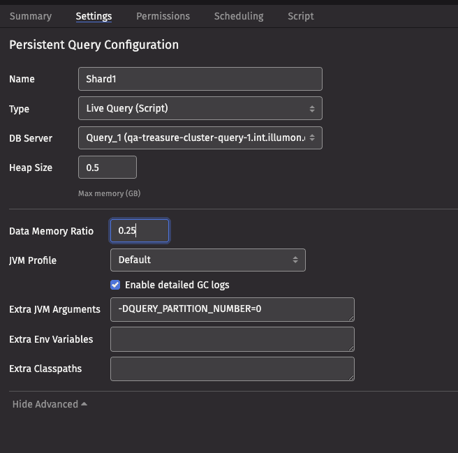
One effective way of setting a QueryScope parameter is to use JVM system properties added to your extra JVM arguments in the query configuration. For example, in the following script the QUERY_PARTITION_NUMBER is read from the system property and stored in a variable in the Groovy binding. Each shard of the query can use the same code, with only the query’s configuration changing the behavior.

QUERY_PARTITION_NUMBER=Integer.parseInt(System.getProperty("QUERY_PARTITION_NUMBER"))
t=db.i("FeedOS", "EquityQuoteL1").where("Date=currentDateNy()").renameColumns("Symbol=LocalCodeStr").where("abs(Symbol.hashCode()) % 4 == QUERY_PARTITION_NUMBER")
symbols=t.selectDistinct("Symbol")

A Java property can also be retrieved from Python:

javaSystem = jpy.get_type("java.lang.System")
javaSystem.getProperty("QUERY_PARTITION_NUMBER")
QUERY_PARTITION_NUMBER=int(javaSystem.getProperty("QUERY_PARTITION_NUMBER"))
t=db.i("FeedOS", "EquityQuoteL1").where("Date=currentDateNy()").renameColumns("Symbol=LocalCodeStr").where("abs(Symbol.hashCode()) % 4 == QUERY_PARTITION_NUMBER")
symbols=t.selectDistinct("Symbol")

The advanced options of the Settings panel in the Query Monitor allows you to set system properties:

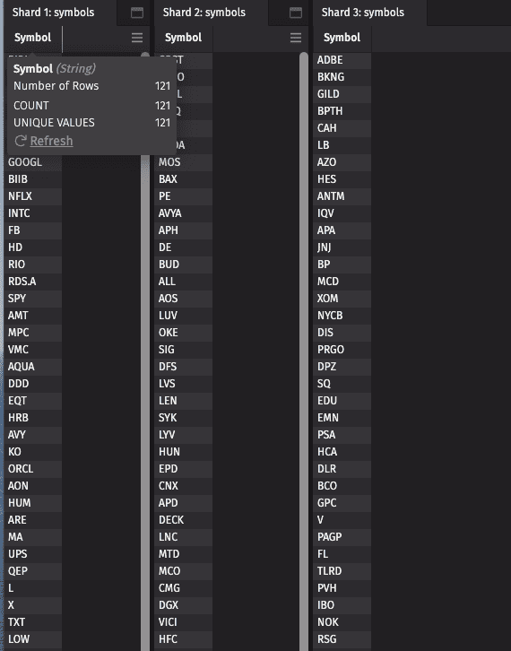
Each query will have a disjoint set of symbols in the table “Symbol”:

where clauses are an effective technique when your data is not already naturally partitioned, and you are operating the query in distinct JVMs. Each input row is processed in each JVM, but the only additional state that must be maintained is the Index that identifies the responsive rows for downstream operations. Each JVM must read the entire data set for columns required to execute the where() clause, and very likely must read the complete raw binary data for other columns as well. This is because Deephaven stores its columns in pages and if the data set is uniformly distributed within the pages, you are likely to require at least one row from each page. Downstream operations need not examine each cell, but the unused data still requires memory and network or disk resources.

Fetching a Specific Internal Partition

If the data is already naturally partitioned, you may be able to use those partitions for your parallelization. For intraday tables, the Database.getIntradayPartitions call provides a list of the internal partitions for the table. You can then use the three argument form of Database.getIntradayTable(namespace, tablename, internalPartitionValue) to retrieve one partition of data. This has the advantage of not requiring any additional filtering, and the query does not need to read extraneous data.

To use internal partitioning to shard your query, care must be taken at the data sources. In particular, for queries that combine data sources, you should ensure that the internal partitioning is consistent among the data sources. When the partitioning is not consistent, you should select the source which drives the queries performance and then use that source’s natural partitioning. The other data sources must then be filtered (across all relevant partitions) to match the primary data source’s partitioning scheme.

TableMaps

The Deephaven API is centered on the Table. A TableMap is a collection of Tables, each with a key. A TableMap allows the query writer to divide a table into segments. The most common method of creating a TableMap is to use the Table byExternal method, which divides a table into a collection of subtables using a set of key columns. For example, to divide the table “t” by the USym and Expiry columns, you could call t.byExternal(“USym”, “Expiry”).

The byExternal call has the advantage over the equivalent iterative where clauses in that the USym and Expiry columns need only be evaluated once, no matter how many combinations of keys and values exist. Moreover, the set of possible keys need not be known in advance; the TableMap interface provides the ability to listen for newly created keys or key-Table pairs.

A simple way of partitioning a Table is to use the hashCode of your query’s partitioning key. For example, on each of your source tables you could divide them by the hashCode of USym:

N_PARTITIONS = Configuration.getInstance().getIntegerWithDefault("N_PARTITIONS", 1)
mkDataTableMap = mktDataSource.updateView("Partition=abs(Symbol.hashCode()) % N_PARTITIONS").byExternal("Partition"))

The Deephaven engine processes the byExternal operation with a single thread, but once the independent tables are created by the byExternal operation, downstream operations can make use of threads. To enable convenient usage, the TableMap exposes an asTable method; for example:

mktData = mktDataTableMap.asTable()

The asTableBuilder() method provides additional options that allow you to control the safety vs. performance trade-offs of various asTable methods.

The "mktData" table can now be used as if it were any other Deephaven table; for example:

puts = mktData.where(“Parity=`P`”)

The where clause is evaluated independently on each table within the TableMap, and a new TableMap is created and presented as the table “puts”. The TableMap backing "puts" will have one key-Table pair for each table in the original TableMap (even if the result of the where is a zero-sized Table). Continuing the same example, we can operate on both the original "mktData" and the "puts" tables:

calls = mktData.where(“Parity=`C`”)
putRenames = puts.renameColumns(“PutBid=Bid”, “PutAsk=Ask”, “PutBidSize=BidSize”, “PutAskSize=AskSize”, “PutTimestamp=Timestamp”)

The "putRenames" and "calls" tables are backed by TableMaps with a parallel key set, which places each USym into a consistent bucket. Therefore, we can use join operations on the "putRenames" and "calls" tables independently, as follows:

putsWithCalls = putRenames.naturalJoin(calls, “USym,Expiry,Strike”, “CallBid=Bid”, “CallBidSize=BidSize”, “CallAsk=Ask”, “CallAskSize=AskSize”, “CallTimestamp=Timestamp”)

Of particular note, when the AsTableBuilder.sanityCheckJoin option is set to true, the Deephaven engine performs additional work to verify that each join key only exists in one of the constituent tables within the TableMap and that the keys are consistent between the two TableMaps. If you are sure that the keys must be consistent, you can disable join sanity checking for improved performance and memory usage.

Enabling TableMap Parallelism

A Deephaven query operation can be divided into two phases. In the first phase, the query operation is initialized. After a query operation is initialized, then the results are updated as part of the LiveTableMonitor refresh cycle.

The TableMap asTable internally calls the TableMap.transformTables method when performing Table methods. The transformTables method executes a function on each of the source TableMap’s constituents and inserts them into a new TableMap. By default, the transformation functions are executed on the calling thread; however, if you set the TableMap.transformThreads property to a value greater than 1, a global thread pool is used for transforming the constituents. For example, you may pass -DTableMap.transformThreads=4 as an extra JVM argument to parallelize updates four ways.

The Live Table Monitor refresh cycle uses a single thread by default, but can be configured to use multiple threads. Each individual table is refreshed in a single-threaded manner, but independent tables can be refreshed on separate threads. The Deephaven query engine keeps track of the dependencies for each table, and ensures that all of the dependencies of a given table have been processed before processing that table. When a TableMap is created, each of its constituents are independent, and therefore their refresh cycles can proceed in parallel, after the byExternal operation has completed its processing.

To enable multiple threads for the LiveTableMonitor, set the LiveTableMonitor.updateThreads configuration property to a value greater than 1. For example, you may pass -DLiveTableMonitor.updateThreads=8 as an extra JVM argument to parallelize updates eight ways.

Presuming your application-level partitions are roughly equal in size, a best practice is to make the number of application-level partitions and the number of transformation or LTM threads equal. If the number of partitions is less than the number of threads, then some of the threads will likely be idle (because there are fewer independent tables than the number of threads). On the other hand, if you chose to use four threads, but five roughly equal partitions, it is very likely that the first four independent tables are processed concurrently, followed by the fifth table - resulting in execution that takes almost twice as than long as if you chose to match the number of partitions to the number of update threads. If the number of independent tables is set much higher than the number of threads, then the additional overhead of maintaining the additional tables and merging the results may reduce performance.

Advanced Methods to Create TableMaps

The byExternal method requires generating a group of data for each constituent table. In some circumstances, this grouping operation can be almost as expensive as the underlying operation to parallelize. For example, to simply count the number of values by a key, the bulk of the operation is creating a grouping. As the byExternal is a fundamentally single-threaded operation, simply performing the count operation with a single thread would be less expensive than dividing the work into multiple threads.

There are two alternative methods of creating TableMaps that do not involve expensive grouping operations:

SourceTableMaps and
EvenlyDividedTableMaps.

SourceTableMaps represent a source table (as returned by db.i or db.t) with each partition as a constituent of the TableMap. The com.illumon.iris.db.v2.SourceTableMapFactory.forDatabase method creates a SourceTableMapFactory, which can then be used to retrieve the actual SourceTableMap. The SourceTableMap is useful when you know that the internal partitioning of the table matches the desired application-level parallelism boundaries.

For example, the following query creates a TableMap of the LearnDeephaven.StockTrades table:

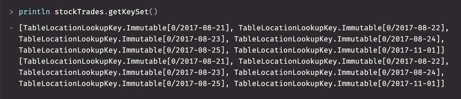
stmf=com.illumon.iris.db.v2.SourceTableMapFactory.forDatabase(db)
stockTrades=stmf.createHistoricalTableMap("LearnDeephaven", "StockTrades")

In this example, Date and internal partition forms a key in the TableMap:

Similarly, an Intraday tablemap can be created for the QueryOperationPerformanceLog:

qoplmap = stmf.createIntradayTableMap("DbInternal", "QueryOperationPerformanceLog", currentDateNy())

It is important to note that the TableLocationKeys for different source tables will not coincide, therefore you will not be able to perform joins between two SourceTableMaps.

The EvenlyDividedTableMap class is useful when you have a Table and simply want to divide it into roughly equal pieces. When using an EvenlyDividedTableMap, it is unlikely that your application-level parallelism boundaries will match your TableMap constituents. Therefore, it is essential that care is taken when combining the results. Moreover, join operations between two evenly divided TableMaps are unlikely to yield the expected results (you may still use an EvenlyDividedTableMap as part of a join operation, but the opposite side should be a Table rather than another TableMap).

Although EvenlyDividedTableMaps support ticking tables, they are currently most effective for static tables. The size of each division is determined at startup, using the initial size of the table, and is not adjusted as the table grows. Additionally, as the table grows or shrinks rows may be moved from one division to another.

Merging Results

In some cases, the TableMap is a suitable result, and it can be exposed to other queries or to UI widgets (such as plots). An asTable result can be converted back to a TableMap with the asTableMap() call. To create a single Table that can be viewed by the UI, or to reaggregate results, the merge() operation should be used.

For example, if we wanted to parallelize a countBy operation across a large Table, we could perform the following operations:

pel = db.i(“DbInternal”, “ProcessEventLog).where(“Date=currentDateNy()”)
peltm = makeEvenlyDividedTableMap(pel, 8, 100000)
counted = peltm.countBy(“N”, “Process”)
merged = counted.merge().sumBy(“Process”)