Empower SQL habits with Deephaven

This document is designed to provide a quick orientation for new Deephaven users who are familiar with SQL relational databases. It should be viewed as a primer on how typical activities are performed in Deephaven versus how they are often performed using SQL. However, it is not meant to be a replacement for the main Deephaven documentation.

Deephaven System Model

Deephaven is a column-oriented database designed for fast and efficient analysis of time-series data. These data may be large volumes of historical information, and/or sets of ticking data where new values are appended as they arrive. Although there are constructs that provide updatable data sets, in a typical installation, greater than 99% of the data will be append-only, immutable values that are being streamed or batch-loaded from some external source.

To better manage the types of information typically stored in Deephaven, its common table type is append-only. In contrast, SQL databases are usually oriented toward the use of Online Transaction Processing (OLTP) with support for Create Read Update Delete (CRUD) actions. For a relational database, a typical table will support adding data anywhere in the table, as well as changing values and deleting rows. This can result in fragmentation and the need for various types of locks within the table. In comparison, a Deephaven data table will be either historical (and thus unchanging), or intraday (where new data is appended to its end). This means no locks are needed to access the on-disk data and no fragmentation can occur. In this way, a Deephaven table is more like the transaction log in a relational database.

Another significant difference between Deephaven and relational database management systems is Deephaven's common use of memory tables. Queries in Deephaven result in in-memory table objects that can contain data, indexes, and formulae. They may or may not have a connection to on-disk data storage. The Deephaven query language includes methods that indicate when data should be populated eagerly into memory versus being read lazily from disk or calculated on the fly. In more complex queries, and in many of the examples in this document, it is common to create tables entirely in memory.

Although they are append-only, Deephaven tables can still be used to track transactional updates. The easiest way for this to work is for update and delete operations to be modeled as appended events to a table: i.e., an update to a row can be written as a new row with the same, for example, row_id (or record_id, etc.) value as the old row, but an incremented version field; and a delete can be a "delete" event appended and referring to the row_id that was deleted. Deephaven provides a powerful and efficient lastBy() command that can then be used to get the latest information for all rows by row_id.

Deephaven also provides a construct called an Input Table that does support CRUD operations. These are intended for relatively small datasets, typically with limited scope, that are used to control queries or extend base sets of data.

SQL Server and Deephaven both provide services for task management, including task scheduling and conditional execution of dependency tasks. In SQL Server, this is the SQL Server Agent; in Deephaven, this role is filled by the Deephaven Controller service.

Query Basics and Order of Processing

Note: Deephaven uses case-sensitive evaluation throughout its processing, so all table names, column names, command names, etc., are case-sensitive.

In most SQL databases, there is a query preprocessor or optimizer that constructs a plan for the execution of the query. This component will usually look at things like indexes, selectivity, and the sizes of involved structures to determine which parts of the query should be processed first. Although useful (and improving with each generation of product), this approach has drawbacks. Index and table statistics are not always up-to-date. Even when they are, the system may make the wrong decision when confronted with an atypical query.

Deephaven instead relies on the user to indicate exactly how the query should be executed. Queries are executed from first to last and left to right. This gives the query author great control, but it also means the system will not correct for unnecessary processing.

In a relational database, a join clause usually comes first. But a join between two tables where a later WHERE clause limits the table to only a few rows will result in the query optimizer applying the WHERE first, before joining the filtered results. In Deephaven, for best efficiency, the query should be written with the where method first, and the join later.

Data Types

Basic Expressions

Deephaven has two concepts of tables: in-memory tables are represented by table variables, and on-disk tables are organized within Deephaven namespaces. Namespaces and on-disk tables are discussed in more detail in Catalog and Metadata.

In-memory representations of tables using table variables are sometimes created using db.t or db.i and other times are created using emptyTable(). Often, when using emptyTable(), the built-in index value, i, is used to populate data values. The emptyTable() method and the i index value are discussed in more detail in Creating Tables.

The basic forms of these two commands follow:

[table_variable] = db.t("[namespace]", "[on_disk_table_name]")
     .where("[partitioning_criteria]")

[table_variable] = emptyTable([number_of_rows])

[table_variable] = db.t("[namespace]", "[on_disk_table_name]")\
     .where("[partitioning_criteria]")

[table_variable] = ttools.emptyTable([number_of_rows])

Immediate Results

SQL dialects usually have a command like Print to return an immediate result. In many implementations, SELECT can also be used for this purpose.

Deephaven query consoles support Groovy and Python. When using Groovy, println can be used to return immediate results or evaluate an expression. When using Python, print is the equivalent.

println "Hello"

2019-02-05 16:25:17.380 STDOUT Hello

print("World")

2019-02-05 16:25:58.422 STDOUT World

Null Handling

In Deephaven, object types inherently support nullability, and primitive types (such as long) support nullability by reserving the minimum value as a "null" value. The null values are available from the QueryConstants class, and are automatically loaded into the Deephaven worker environment. They have names like NULL_INT for the integer value used to represent null. Using these reserved values to track nulls in primitive data types allows them to support nulls and still remain small and efficient to work with, at the cost of one less value in their ranges of possible values.

To verify whether a primitive value is null requires use of the following constants, or the isNull() operator.

x == null        // this does not work to check for a null integer

isNull(x)        // this is preferred

x == NULL_INT    // this also works, but it requires that the type of x is known to be int

x == None        # this does not work to check for a null integer

x is None        # this is preferred

This is similar to the use of IS NULL in many SQL dialects.

Literal Values

In script code, both Groovy and Python use double quotes to delimit string literals. For example:

x="Hello"

y="World"

Within Deephaven query expressions, the backtick (`) is used instead of a double quote because double quotes are already being used to delimit the query expression. For example:

.update("Column1=`Hello World`")

Single ticks (single quotes) are used within Deephaven queries to delimit DBDateTime values. For example:

q2=Quotes.where("ExchangeTimestamp='2017-08-25T04:00:00.071175597 NY'")

String Manipulation

Deephaven Strings support Java String methods.

Concatenation in Deephaven is similar to SQL.

t1 = emptyTable(1).update("Col1 = `Hello` + ` ` + `World`")

from deephaven import *

t1 = ttools.emptyTable(1).update("Col1 = `Hello` + ` ` + `World`")

Concatenating a String with a numeric type will automatically convert the number to String. Concatenating a non-null String with a null will convert the null to the literal value "null".

Other commonly used methods include the following:

• .substring(start, end)

• .replace(pattern_to_find, pattern_to_replace)

• .toUpperCase() and .toLowerCase()

• .length()

• .contains(pattern_to_find) // true or false

• .indexOf(pattern_to_find) // starting offset of first match

• .reverse()

Datetimes

Deephaven's DBDateTime data type use a long (64-bit) value to represent nanoseconds (plus or minus) from epoch (January 1, 1970 at midnight GMT). DBDateTimes can range from September 21, 1677 to April 12, 2262.

A new DBDateTime can be instantiated at epoch with the following:

dbt=new DBDateTime()

from deephaven import *

dbt = dbtu.currentTime()

A new DBDateTime can be instantiated from a value of epoch offset nanosecond with the following:

dbt=new DBDateTime([long_value_in_nanoseconds])

from deephaven import *

dbt = dbtu.nanosToTime([long_value_in_nanoseconds])

Offset values from epoch can be obtained from DBDateTimes using .getNanos() or .getMillis().

To make these offset values easier to work with, Deephaven provides the following constants:

• SECOND
• MINUTE
• HOUR
• DAY

For example, a DBDateTime could be constructed using the following constants:

dbt=new DBDateTime(15 * YEAR + 15 * DAY + 6 * HOUR + 30 * MINUTE)

from deephaven import *

dbt = dbtu.nanosToTime(15 * dbtu.YEAR + 15 * dbtu.DAY + 6 * dbtu.HOUR + 30 * dbtu.MINUTE)

The previous query returns the following:

1985-01-12T01:30:00.000000000 NY

Note: The results show January 12, 1985 because three leap years occurred between 1970 and 1985. The YEAR constant is the same as 365 days worth of nanoseconds.

For string and literal representations of datetimes, Deephaven uses a variant of ISO format:

yyyy-mm-ddThh-mi-ss.mmmmmmnnn TZ

This can be seen in the example above, and can also be used with the convertDateTime() static method to convert a String to a DBDateTime:

dbt=convertDateTime("1985-01-12T01:30:00.000 NY")

from deephaven import *

dbt = dbtu.convertDateTime("1985-01-12T01:30:00.000 NY")

See the Temporal Data section in the full Deephaven documentation for more information on working with temporal data.

WHERE is filtering, JOIN is not

In relational databases, an inner join is often used to filter a large data set to few interesting values. In the Deephaven Query Language, where, and its variants, are used for filtering, but join operators are fundamentally used to combine data from multiple tables, and are not optimized for filtering.

In SQL, the following two statements are equivalent:

SELECT c.*
FROM Customers c
     INNER JOIN MyCustomers m
     ON c.customer_id = m.customer_id

SELECT *
FROM Customers
WHERE customer_id IN (SELECT customer_id FROM  MyCustomers)

In DQL, the following two statements are comparable:

myResult = Customers.join(MyCustomers, "customer_id")

myResult = Customers.whereIn(MyCustomers, "customer_id")

However, the internal processing between these two is very different. The second Deephaven query, using whereIn(), will accomplish the desired filtering of data by reading only rows from Customers that have matching values in MyCustomers. The first Deephaven query will read all customer_ids from Customers into memory, and all customer_ids from MyCustomers, and will then proceed to join rows on matching values. This works well if most or all rows from Customers are needed. However, it is common for Deephaven tables to have hundreds of millions of rows, and all of those values may not fit into the memory allocated to the query Worker.

Since myResult does not need any data from MyCustomers, using whereIn() is the correct method to use the contents of MyCustomers to filter data from the Customers table.

Sorting and Limiting Result Sets

Sorting

Sorting in Deephaven is similar to sorting in SQL, except for when the sort is to be performed.

• In SQL, an ORDER BY clause goes at the end of a statement, but may be applied to the results before other clauses earlier in the query.
• In Deephaven, the processing of clauses is always first-to-last/left-to-right. So, if a result set needs to be sorted before some other processing can or should be applied, the sorting clause also needs to be placed earlier in the query.

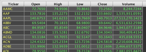
In Deephaven, sort() is the equivalent of ORDER BY and sortDescending() is the same as ORDER BY … DESC. Multiple columns can be passed to the sort methods to be used for sub-sorts in the same direction.

An example query and the resulting table follows:

Prices=db.t("LearnDeephaven","EODPrices").where("ImportDate=`2017-11-01`")
sortedOpenDesc=Prices.sortDescending("Ticker","Open")

from deephaven import *

Prices=db.t("LearnDeephaven","EODPrices").where("ImportDate=`2017-11-01`")
sortedOpenDesc=Prices.sortDescending("Ticker","Open")

When processing a sort, Deephaven preserves the order of the data it receives other than explicitly requested ordering for the current sort operation. This allows multiple sorts to be used to set cascading levels of sorting in different directions.

Consider the following in SQL:

SELECT *
FROM Prices
ORDER BY Ticker DESC, Open ASC

This would be equivalent to the Deephaven query below (sorting in descending order by Ticker does not change the order of values already sorted within Tickers by Open):

sortedMixed=Prices.sort("Open").sortDescending("Ticker")

Head and Tail

Relational databases usually provide a method to return only a subset of matching data. In T-SQL this is done with TOP, where as LIMIT is the operator in MySQL.

In Deephaven, head() and tail() are provided to return the first or last (respectively) subset of rows. The headPct() and tailPct() methods are also provided for percentage-based limiting.

T-SQL Example:

SELECT TOP 10 Ticker, Close
FROM EODPrices
ORDER BY Close DESC

MySQL Example:

SELECT Ticker, Close
FROM EODPrices
ORDER BY Close DESC
LIMIT 10

Deephaven Example:

mostExpensive=db.t("LearnDeephaven","EODPrices")
        .where("ImportDate=`2017-11-01`")
        .sortDescending("Close")
        .head(10)
        .select("Ticker","Close")

from deephaven import *

mostExpensive=db.t("LearnDeephaven","EODPrices") \
    .where("ImportDate=`2017-11-01`") \
    .sortDescending("Close") \
    .head(10) \
    .select("Ticker","Close")

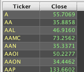
In the SQL and Deephaven versions of the query, a sort is required to tell the system which rows are at the top and should be returned. However, the order of statements in the Deephaven query: limiting/filtering with head is done before selecting the column values, so the query will only need to retrieve the Ticker values for the ten rows that correspond to the ten highest values in the Close column. Also, the sort must happen before head() limits the rows. If head() were used before sort() in the Deephaven query, the system would retrieve whatever ten rows it first found, then sort those ten rows in descending order by the value in the Close column.

For example:

Deephaven table generated using sortDescending first:	Deephaven table generated using head(10) first:

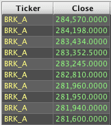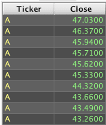Aggregation

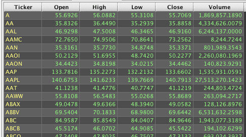
Deephaven has a comparable set of aggregation functions to those available in most SQL implementations, including sum(), average(), count(), etc. However, their use in Deephaven is different than in SQL. In SQL, a column or expression is passed to an aggregate function, and the function creates a new column as a result. For example:

SELECT AVG(Close) AS Avg_Close
FROM Prices

The above query creates an overall average of Close values for the entire Prices table. If averages are desired for specific subsets of data from the Prices table, a GROUP BY clause must be added, usually along with the grouping value to display in the results, as shown below:

SELECT
     Ticker,
     AVG(Close) AS Avg_Close
FROM Prices
GROUP BY Ticker

In Deephaven, the syntax is essentially reversed. The aggregate function is passed to the grouping column(s), and will then operate on every remaining column in the table. For example, the following query fails, because it is trying to average each of the columns in the table, including the String column, Ticker.

Prices=db.t("LearnDeephaven","EODTrades").where("ImportDate=`2017-11-01`")
myResult=Prices.avgBy()

from deephaven import *

Prices=db.t("LearnDeephaven","EODTrades").where("ImportDate=`2017-11-01`")
myResult=Prices.avgBy()

To get an overall average, the methods select() or view() must be used to restrict the table to just the Close column:

myResult=Prices \
    .view("Close") \
    .avgBy()

Or, the following query can be used to get average values by ticker:

myResult=Prices \
    .select("Ticker","Close") \
    .avgBy("Ticker")

Other columns in the table that are passed to the aggregate function will also be aggregated as long as they are compatible data types. In the following example, the values in the Open, High, Low, and Volume columns are all numeric, so they can also be processed by avgBy().

myResult=Prices \
    .select("Ticker","Open","High","Low","Close","Volume") \
    .avgBy("Ticker")

Because Deephaven allows multiple operations to be applied when creating a result, a HAVING clause is not needed for aggregation. Instead, a where() filter is executed after the aggregate to accomplish the same type of post-aggregation filtering. A sample query and its resulting table follows:

myResult=Prices \
    .select("Ticker","Open","High","Low","Close","Volume") \
    .avgBy("Ticker") \
    .where("Open > 60")

Combining Result Sets

Many SQL dialects provide a union operator to combine multiple result sets that have the same number and compatible types of columns.

SELECT A, B, C FROM TABLE1 WHERE (X=3)
UNION
SELECT D, E, F FROM TABLE2 WHERE (Q=4)

or

SELECT A, B, C FROM TABLE1 WHERE (X=3)
UNION ALL
SELECT D, E, F FROM TABLE2 WHERE (Q=4)

The difference between these two is that UNION will eliminate duplicate rows, and UNION ALL will leave them in the final results.

The comparable method to UNION ALL in Deephaven's query language is merge(). Its results and behavior are similar to UNION ALL, but its application is rather different. First, using merge() requires matching column names and matching data types. Also, merge() is called once and is then passed multiple tables to combine rather than being called multiple times.

The following Deephaven query is comparable to the SQL UNION ALL example above:

result=merge(
        table1.where("X=3").view("A","B","C"),
        table2.where("Q=4").view("A=D","B=E","C=F"))

from deephaven import *

result=ttools.merge(
    table1.where("X=3").view("A","B","C"),
    table2.where("Q=4").view("A=D","B=E","C=F"))

In this example, view("[newName1]=[oldName1]",..."[newNamen]=[oldNamen]") is used to rename the columns while also constraining which columns are included in the resulting table to be merged. The select() method also supports the same syntax, but, as mentioned earlier, select() will load the column data into memory eagerly, while view() will load it lazily.

The renameColumns() method can also be used to rename one or more columns in a table, without retrieving them into memory. The syntax follows:

renameColumns("[newName1]=[oldName1]",..."[newNamen]=[oldNamen]")

For example:

table2=table2.renameColumns("A=D","B=E","C=F")

lastBy and Downsampling

Because Deephaven is optimized for time series data, there are built-in capabilities that make it very easy to manipulate information based on its timestamp or sequence. A particularly important example is lastBy(). SQL has no single command that is comparable.

The lastBy() method is an aggregation function that returns the last values, by the specified grouping columns, according to the sorted order of the table. Because most data in Deephaven is appended to a table based on occurring events, the default result of a lastBy() will provide the most recent values for the grouping keys.

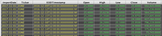
For example, the following query generates the initial Prices table, and then uses lastBy() to show the most recent row from the Prices table for each symbol:

Prices=db.t("LearnDeephaven","EODPrices").where("ImportDate=`2017-11-01`")
lastPrices=Prices.lastBy("Ticker")

from deephaven import *

Prices=db.t("LearnDeephaven","EODPrices").where("ImportDate=`2017-11-01`")
lastPrices=Prices.lastBy("Ticker")

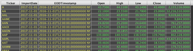
Doing the same thing in SQL would usually require a correlated sub-query, or derived sub-table. For example:

SELECT *
FROM Prices p1
WHERE EODTimestamp =
     (    SELECT
              MAX(EODTimestamp)
          FROM Prices p2
          WHERE p2.Ticker = p1.Ticker)

or

SELECT Prices.*
FROM Prices
     JOIN (     SELECT
                    Ticker, MAX(EODTimestamp) AS EODTimestamp
                FROM Prices
                GROUP BY Ticker) MaxTS
     ON Price.Ticker = MaxTS.Ticker
  AND Price.EODTimestamp = MaxTS.EODTimestamp

This assumes the EODTimestamp values are unique for each Ticker value; otherwise, SQL would require additional logic to limit to one "last" value per symbol.

Deephaven's binning functions make it fairly easy to downsample large volumes of time series data. They can be used in conjunction with lastBy() or the aggregate functions to obtain a lower resolution view of detailed data.

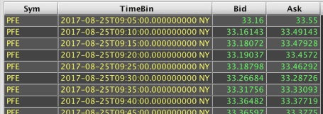
For example, this statement generates the initial Quotes table:

Quotes=db.t("LearnDeephaven","StockQuotes").where("Date=`2017-08-25`")

The following is then applied to return the last row for each five-minute interval for each symbol's quote data:

dsQuotes=Quotes \
    .update("TimeBin=lowerBin(ExchangeTimestamp, 5*MINUTE)") \
    .lastBy("Sym","TimeBin")

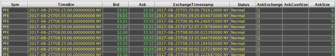
The update() portion of the query adds a TimeBin column that will be the beginning of a five-minute interval, on the five-minute mark, that contains the row's data. The lastBy() then filters to only the last row for each unique Sym and TimeBin value combination.

In most dialects of SQL, adding the TimeBin would require datetime parsing or some other work, either in the query expression or in a user-defined function, to construct the rounded time window value. The following demonstrates this using SQL Server's T-SQL:

DECLARE @today DATETIME
SET @today = DATEADD(Day, DATEDIFF(Day, 0, GETUTCDATE()), 0)

SELECT *,
     DATEADD(Minute,
     (DATEDIFF(Minute, @today, exchange_timestamp)
           - DATEDIFF(Minute, @today, exchange_timestamp) % 5),
     @today) AS timebin
FROM Prices

Note that upperBin and firstBy are also available in Deephaven. The upperBin() method makes a timestamp that corresponds to the end of the specified window, and firstBy() retrieves the first matching value in the range.

Rather than sub-sampling, averaging in Deephaven can be done using the avgBy() method as shown below:

dsAvgQuotes=Quotes \
    .update("TimeBin=lowerBin(ExchangeTimestamp, 5*MINUTE)") \
    .select("Sym","TimeBin","Bid","Ask") \
    .avgBy("Sym","TimeBin")

Deephaven Tables vs. SQL Views

Deephaven tables are similar to SQL views, in that they both provide presentations of data. This presentation is formed using a query that might join data from multiple sources, manipulate and filter information, sort values, and perform other operations such as binning. Where the two start to differ is in terms of what they store.

Some SQL implementations offer materialized views, which are views that store their own data rather than executing a query when needed and pulling the results from that. Deephaven tables offer the query author options about whether to store data or retrieve/calculate it when needed, on a column-by-column basis.

Consider the following query in SQL:

CREATE VIEW MyQuotes
AS
SELECT
    Sym,
    Bid,
    Ask,
    ExchangeTimestamp
FROM Quotes
WHERE Sym IN ('AAPL','SPY','VMW')

MyQuotes does not store any data. Instead, its query will be effectively executed as a derived sub-table when a query is run against it, such as the following:

SELECT
     Sym,
     AVG(Bid) AS AvgBid
FROM MyQuotes
WHERE Bid > 30
GROUP BY Sym

In Deephaven, statements such as select(), view(), update(), updateView(), and lazyUpdate() indicate to the query engine whether to store data (similarly to a materialized view, or temp table) or to calculate/fetch data when needed (like a regular SQL view).

For example, consider the following Deephaven script:

Quotes=db.t("LearnDeephaven","StockQuotes").where("Date=`2017-08-25`")

myQuotes1=Quotes
        .where("Sym in `AAPL`,`SPY`,`VMW`")
        .select("Sym","Bid","Ask","ExchangeTimestamp")
        .update("TimeBin=lowerBin(ExchangeTimestamp, 5*MINUTE)")

myQuotes2=Quotes
        .where("Sym in `AAPL`,`SPY`,`VMW`")
        .view("Sym","Bid","Ask","ExchangeTimestamp")
        .updateView("TimeBin=lowerBin(ExchangeTimestamp, 5*MINUTE)")

from deephaven import *

Quotes=db.t("LearnDeephaven","StockQuotes").where("Date=`2017-08-25`")

myQuotes1=Quotes \
    .where("Sym in `AAPL`,`SPY`,`VMW`") \
    .select("Sym","Bid","Ask","ExchangeTimestamp") \
    .update("TimeBin=lowerBin(ExchangeTimestamp, 5*MINUTE)")

myQuotes2=Quotes \
    .where("Sym in `AAPL`,`SPY`,`VMW`") \
    .view("Sym","Bid","Ask","ExchangeTimestamp") \
    .updateView("TimeBin=lowerBin(ExchangeTimestamp, 5*MINUTE)")

In this case, myQuotes1 and myQuotes2 both return the same data.

In myQuotes1, select() and update() are used. The select() operation retrieves and stores in memory the column values that match the where() clause; and update() proactively calculates and stores the lowerBin() values for all rows in the table. On the other hand, myQuotes2 uses view() and updateView(). The view() operation tells the query engine to retrieve the column values when needed (for display or for another query) rather than initially loading and keeping them in memory. The updateView() operation indicates the TimeBin value will be calculated when needed for corresponding rows, rather than being generated for all the rows up front.

In this example, myQuotes2 acts more like a regular SQL view, and myQuotes1 acts more like a materialized view. Using the methods demonstrated in myQuotes2 would be better in situations where not all of the rows will be used or when memory is scarce. However, using the methods demonstrated in myQuotes1 would be better in situations where all rows will be accessed, especially when some rows will be accessed multiple times.

In addition, the lazyUpdate() option allows a blend of update() and updateView(). The lazyUpdate() method will calculate values on demand, like updateView(), but will cache the calculated values. This is particularly useful when input data added to a calculated column has a small number of distinct values and memory is scarce.

Data Organization

In most SQL databases, data is stored in monolithic binary files. Table, column, and index data may be dispersed throughout a file and also spread across multiple files. Deephaven makes more direct use of the filesystem on which it is running to manage organization of tables and columns. For instance, column data for a particular table and partition in Deephaven is stored in files whose names match the column name. This is described in detail in the Table Storage topic in the main Deephaven documentation.

The main point of relevance relative to relational databases is that, to retrieve a single column in an efficient manner, a relational database normally needs a non-clustered index to store this column data separately from the table itself. In Deephaven, the column data is already separated by its native storage.

Partitions

The term "partition" has different meanings in Deephaven, depending on the context.

For intraday tables, internal partitions describe different sources for streaming data. For example, there may be multiple feeds of options data populating the same intraday table. These internal partitions correspond to distinctly named directories in the hierarchy of directories that store intraday data for a table. Deephaven will coalesce data from these directories when presenting intraday data from all of them to the user.

For historical tables, partitions are first configured; then large sets of table data can be separated during the merge process. These are usually physical partitions so large tables can leverage multiple storage devices for faster access and higher throughput.

For both types of tables, there is also a partition called the column partition, which refers to how data in the table is physically and logically separated. Data is most commonly separated by date (when the data was received), but data can be partitioned by any unique String value. When a query is executed, either for intraday data (with db.i) or for historical data (with db.t), the system will expect a where() clause to be included. Best performance is obtained if that where() clause limits retrieved data to a specific partition or limited set of partitions. This is because the partition corresponds to one or a small set of directories on the filesystem, thus minimizing the work the query engine needs to do to find the subsets of table data that will be of interest for the query.

The last type of partitioning is of most interest to the table designer and query writer. In relational databases, it is often possible to create horizontally partitioned tables, where the "table" that users use is actually a view that unions data from multiple sources. The separation of intraday data by column partition value in Deephaven basically forces this type of a design, but also automates most of its use. This is one of the ways Deephaven achieves highly responsive query execution against datasets where a single day often adds as many rows as are contained in the largest tables in most relational databases.

Grouping

Grouping is specified in the schema when a table is created, but it applies only to historical tables. In relational databases, grouping typically refers to how groups are formed when aggregating data and calculating subtotals, sub-averages, etc. In Deephaven, grouping determines which sets of rows should be kept together when they are written to physical partitions during the merge process. Optional sorting can also be applied to the data during the merge process.

Although not an exact equivalent, Deephaven's arrangement of data during merge is similar to a clustered index on a relational table. Both control how data will be physically organized on the storage media, and both work best when the grouping and sorting columns are chosen based on how sets of data are most commonly retrieved.

Indexes

Indexes in Deephaven are entirely different structures than indexes in relational databases. Deephaven indexes are simply integer (32-bit) or long (64-bit) values for finding and accessing rows. When working with ticking data, these indexes are ephemeral, and user-visible values for them are likely to change when new data is added to the table.

In Deephaven, there are no data access indexes that need to be created or specified to achieve good query performance..

More information about Deephaven indexes and their use can be found in the Array Access documentation.

Join Types

As mentioned earlier, join operations in Deephaven are designed to extend result sets by incorporating data from other tables. Unlike relational databases, Deephaven joins are not intended to filter data. An inner join will filter data, but it will do so after loading all keys from the source tables into memory, which may result in higher memory utilization than is necessary or desirable.

Inner Join

The Deephaven join() operator is logically very comparable to INNER JOIN in ANSI SQL. It matches rows from two tables based on specified keys. The basic join() syntax in Deephaven follows:

resultTable=leftTable.join(rightTable, "Key1, … Keyn")

For ANSI SQL the syntax would be:

SELECT *
FROM leftTable
INNER JOIN rightTable
ON leftTable.Key1 = rightTable.Key1
    AND … leftTable.Keyn = rightTable.Keyn

A join() executed where the key values for all rows match will return a Cartesian product, i.e., a CROSS JOIN in SQL.

There are some minor differences between the SQL and Deephaven inner join behaviors. The Deephaven join() operator takes an optional third argument, which allows specifying which columns from the right table to include in the result set. If this argument is omitted, the join() operation will exclude the matched key column(s) of the right table from the result set, but include all other columns. For example:

leftTable=emptyTable(5).update("Row=i","leftData=100+i*3")
rightTable=emptyTable(10).update("Row=i","rightData=`A`+i")

result=leftTable.join(rightTable,"Row")

Internally, join() executes naturalJoin() plus some additional logic. If the needed result can be obtained from naturalJoin(), that will be the more efficient and recommended solution.

Array Left Join

Deephaven's query language includes a leftJoin() method. As the name implies, this operation performs a LEFT OUTER JOIN match between left and right tables. This method differs from an ANSI SQL LEFT OUTER JOIN as leftJoin() will always return one row for each row in the left table. If there is no match in the right table, then right table cells will contain nulls. If there are any matches, then the right table cells for matching rows will have arrays of results.

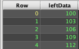
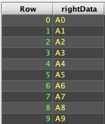
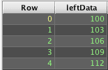
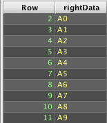
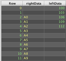
Consider the following Deephaven query:

leftTable=emptyTable(5).update("Row=i","leftData=100+i*3")
rightTable=emptyTable(10).update("Row=(i*2%5)+2","rightData=`A`+i")

result2=leftTable.leftJoin(rightTable,"Row")

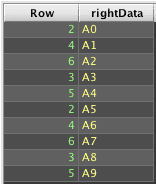
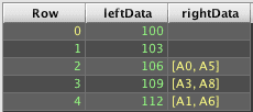
To obtain results similar to those produced by a ANSI LEFT OUTER JOIN in SQL requires ungrouping the array results. However, the unmatched right side cells contain only nulls, not arrays of null, so just ungrouping result2 will drop the unmatched rows:

ungroup=result2.ungroup()

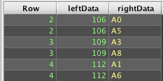
Instead, the rightData column must first be modified to contain a consistent data type - arrays of String in this case:

leftOuterJoin = leftTable.leftJoin(rightTable, "Row")
        .update("rightData = isNull(rightData) ? new String[]{null} : rightData.toArray()")
        .ungroup()

from deephaven import *

leftOuterJoin = leftTable.leftJoin(rightTable, "Row") \
    .update("rightData = isNull(rightData) ? new String[]{null} : rightData.toArray()") \
    .ungroup()

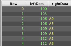
The toArray() portion of this update is needed to convert the DBArray type that leftJoin() returned for matching rows' cells to a regular String[], which is the same type that new String[]{null} will fill in for null cells.

Natural Join

The Deephaven naturalJoin() operator is similar to SQL's OUTER JOIN, or, more specifically, LEFT OUTER JOIN, in that it will return matching rows between the left and right tables, and will return nulls in the columns of the right table for left table rows that do not have a match in the right table.

Deephaven's naturalJoin() differs from a SQL OUTER JOIN; it will fail if there are multiple right table matches for a left table row's keys. For example:

leftTable=emptyTable(5).update("Row=i","leftData=100+i*3")
rightTable=emptyTable(10).update("Row=i+2","rightData=`A`+i")

result=leftTable.naturalJoin(rightTable,"Row")

Deephaven's query language does not include right outer join operators. However, like SQL, switching the tables in a LEFT OUTER JOIN returns the same results as a RIGHT OUTER JOIN.

To accomplish the same thing as a SQL OUTER JOIN in cases where there may be multiple matching right table rows, please refer to the Array Left Join topic above.

How to Perform a FULL OUTER JOIN

In ANSI SQL, a FULL OUTER JOIN returns all matching rows, including Cartesian matches, and all non-matched rows with nulls in the columns from the "other" table, e.g., parent processes with child processes, parent processes that have no child processes, and orphaned child processes.

The SQL form of such a query follows:

SELECT *
FROM leftTable
     FULL OUTER JOIN rightTable
     ON leftTable.Row = rightTable.Row

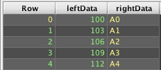
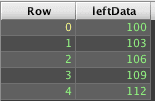
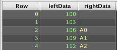
Deephaven's query language does not have a directly comparable join operation. Instead, a combination of commands is needed to use leftJoin() to build the full outer join result set:

leftTable=emptyTable(5).update("Row=i","leftData=100+i*3")
rightTable=emptyTable(10).update("Row=i+2","rightData=`A`+i")

distinctRows=merge(leftTable.selectDistinct("Row"), rightTable.selectDistinct("Row"))
        .selectDistinct("Row")

fullOuterJoin=distinctRows
        .leftJoin(leftTable, "Row")
        .update("leftData = isNull(leftData) ? new int[]{NULL_INT} : leftData.toArray()")
        .ungroup()
        .leftJoin(rightTable, "Row")
        .update("rightData = isNull(rightData) ? new String[]{null} : rightData.toArray()")
        .ungroup()

from deephaven import *

distinctRows=ttools.merge(leftTable.selectDistinct("Row"), rightTable.selectDistinct("Row")) \
    .selectDistinct("Row")

fullOuterJoin=distinctRows \
    .leftJoin(leftTable, "Row") \
    .update("leftData = isNull(leftData) ? new int[]{NULL_INT} : leftData.toArray()") \
    .ungroup() \
    .leftJoin(rightTable, "Row") \
    .update("rightData = isNull(rightData) ? new String[]{null} : rightData.toArray()") \
    .ungroup()

This is similar to the left outer join example under the Array Left Join topic. However, this example starts by creating a table of unique Row (key) values across the left and right tables, and then uses that table as the left table for a left outer join to get the matched and unmatched rows. Because this uses leftJoin() for its processing, it also allows cases where there are multiple matches from either side.

As-of Joins and Reverse As-of Joins

Deephaven's As-of Joins and Reverse As-of Joins — aj() and raj() respectively — provide functionality specific to joining data based on the proximity of timestamps when events occurred, as opposed to exact matches of relational join keys. This is an area where SQL requires multiple statements to implement the same logic of a single Deephaven statement.

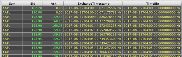
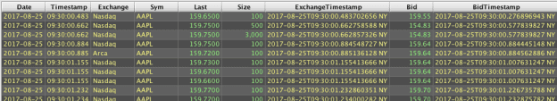
The following Deephaven query statements set up tables with stock quote and trade data for AAPL on August 25th, 2017. (Note: some columns have been omitted in the screenshots to make the results more obvious.):

Trades=db.t("LearnDeephaven","StockTrades")
        .where("Date=`2017-08-25`","Sym=`AAPL`","SaleCondition=`@`")
        .dropColumns("SaleCondition","Source","ExchangeId","USym","SecurityType")

Quotes=db.t("LearnDeephaven","StockQuotes")
        .where("Date=`2017-08-25`","Sym=`AAPL`")

from deephaven import *

Trades=db.t("LearnDeephaven","StockTrades") \
    .where("Date=`2017-08-25`","Sym=`AAPL`","SaleCondition=`@`") \
    .dropColumns("SaleCondition","Source","ExchangeId","USym","SecurityType")

Quotes=db.t("LearnDeephaven","StockQuotes") \
    .where("Date=`2017-08-25`","Sym=`AAPL`")

An As-of Join can then be used to show the bid price of the most recent quote at or before each trade:

LastQuote=Trades.aj(Quotes,"ExchangeTimestamp","Bid, BidTimestamp=ExchangeTimestamp")

The aj() method is similar to the other join methods, in that it takes a table to join to, one or more join keys, and, optionally, a list of columns to add to the resultant table. If the third argument is omitted, all columns except the join columns are added. If there is no match from the right table for a left table row, null values are included for the columns from the right table in the resultant row.

In the previous example, Bid and ExchangeTimestamp are added, but ExchangeTimestamp is renamed to BidTimestamp.

The raj() — or Reverse As-of Join — method is used in the same way, but will instead join to the first row on or after the left table's row.

The aj() and raj() methods expect to use the sorting of the right table to find the correct row to match. In this example, the Quotes and Trades tables are already sorted by ExchangeTimestamp. Therefore, no additional sorting is needed.

An example of a comparable SQL query follows:

SELECT t.*, q.Bid, q.ExchangeTimestamp as BidTimestamp
FROM Trades t
     JOIN Quotes q
        ON q.ExchangeTimestamp = (
             SELECT MAX(q2.ExchangeTimestamp)
             FROM Quotes q2
             WHERE q2.ExchangeTimestamp < t.ExchangeTimestamp)

As with the lastBy() equivalent, this SQL query will return multiple rows if there are duplicate ExchangeTimestamp values in the Quotes table.

ExactJoin

Deephaven's exactJoin() method is straightforward, but it is not something seen in common SQL dialects. The exactJoin() method expects exactly one match between each left table row and the right table. Any duplicate matches or orphaned rows from the left table will cause the exactJoin() method to fail.

Doing something similar in SQL would require an explicit check, such as the following:

IF EXISTS (SELECT COUNT([ right table join columns ])
          FROM LeftTable
               LEFT JOIN RightTable
                   ON [ join expressions ]
          GROUP BY [ right table join columns ]
          HAVING COUNT([ right table join columns ]) <> 1)
RAISEERROR …

Catalog and Metadata

Namespace and Table Names

A namespace in Deephaven has a number of similarities to a database in SQL Server or MySQL, or a tablespace in Oracle. Namespaces serve to group tables together, and to provide scope in which table names must be unique.

In SQL Server, there are System databases and User databases. Deephaven has System namespaces and User namespaces, but the distinction between the two types of namespaces is a different than the two databases in SQL Server.

Deephaven's System namespaces store their table data under the Systems or Intraday directories under the database root (normally /db) on the query servers. System tables are created by system administrators and have schema files to provide their table definitions.

Deephaven's User namespaces are created directly by users when they create the first user table in a new namespace. By default, users have access to a namespace that matches their username. User tables are stored under the Users directory in the database root.

Available namespaces are automatically presented in a Deephaven console by pressing the Tab key after typing db.i(" or db.t(" in a query.

Deephaven also provides catalog and metadata methods that are analogous to SQL INFORMATION_SCHEMA views or MySQL's SHOW DATABASES and SHOW TABLES commands.

In Deephaven, the following methods each return a list of namespace names:

• db.getNamespaces()

• db.getUserNamespaces()

• db.getSystemNamespaces()

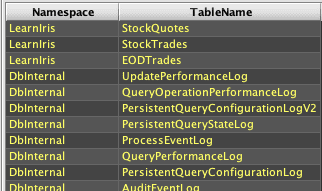
For example, entering println db.getSystemNamespaces() in a Deephaven console will generate the following:

2019-02-05 18:06:08.022 STDOUT [LearnDeephaven, DbInternal, … ]

DbInternal and LearnDeephaven are two special System namespaces.

• DbInternal contains management and monitoring table for Deephaven itself. This is comparable to the master database in SQL Server.
• LearnDeephaven contains example data, which is similar to the pubs or Northwind databases found in SQL Server.

A list of tables available within a Deephaven namespace can be queried using db.getTableNames([namespace]). A list of all available tables across all available Deephaven namespaces can be queried using db.getCatalog().

For example, the following will generate a log output listing the tables within the DbInternal namespace:

println db.getTableNames("DbInternal")

2019-02-06 09:32:28.358 STDOUT [PersistentQueryStateLog, UpdatePerformanceLog, PersistentQueryConfigurationLogV2, PersistentQueryConfigurationLog, QueryOperationPerformanceLog, AuditEventLog, ProcessEventLog, QueryPerformanceLog]

For another example, the following will generates a Deephaven table containing showing the tables within all available namespaces:

catalog=db.getCatalog()

Deephaven's getMeta() method can be used to retrieve table description metadata for table variables. The table variable could have been created by reading a table from disk with db.i or db.t, or it could have been created directly in memory by a variety of methods, or it could be the result of query operations against other tables. Regardless, where a table variable is available, getMeta() can be used to return a new table that contains the table's metadata.

The following Deephaven query retrieves metadata for an in-memory table:

Quotes=db.t("LearnDeephaven","StockQuotes")
        .where("Date=`2017-08-25`","Sym=`AAPL`")
md=Quotes.getMeta()

from deephaven import *

Quotes=db.t("LearnDeephaven","StockQuotes") \
    .where("Date=`2017-08-25`","Sym=`AAPL`")
md=Quotes.getMeta()

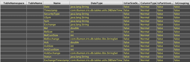
The following Deephaven query retrieves metadata for an on-disk table:

md=db.t("LearnDeephaven","StockQuotes").getMeta()

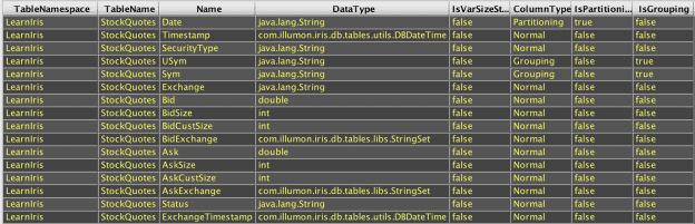
Note that TableNamespace and TableName are blank for the in-memory table, but populated for the on-disk table. The same table schema is being used, but the application of where() filtering in the first example to restrict the table to a particular partition and symbol is the point at which it changes from an on-disk table to an in-memory table.

Creating Tables

Most SQL dialects include the CREATE TABLE statement to create a new persistent table. Some also include options to create table variables for small, in-memory tables.

In Deephaven, there are four main categories of tables:

1. System tables are on-disk tables created by administrators using schema files for table definitions
2. User tables are on-disk tables created by users from within the query language
3. Input tables are on-disk tables created by users from within the query language; requires initial administrative configuration to enable this feature
4. In-memory tables are in-memory tables created by users from within the query language

For all but System tables, the table definition can either be defined column-by-column, or inherited from another table using getDefinition().

In-memory tables are the most commonly used type of table in Deephaven. Like SQL Server table variables, Deephaven's in-memory tables are ephemeral and are released when the Deephaven query worker process exits.

In-memory tables can be created and loaded with data from a number of sources:

• db.i([namespace],[table_name]).where(... creates an in-memory table from an intraday on-disk table
• db.t([namespace],[table_name]).where(... creates an in-memory table from a historical on-disk table
• emptyTable() creates a new memory table with no data
• [table].[some_table_method] creates a new in-memory table from an existing memory table
• readCsv, readBin, and getQuandl are examples of methods that create new in-memory tables while importing data from files or Internet-based data sources

emptyTable

An easy way to create a new in-memory table in Deephaven is by using the emptyTable() method. The emptyTable() method takes one argument: the number of rows to create in the table.

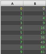
For example, the following creates a table with 10 rows, but no columns.

newTable=emptyTable(10)

from deephaven import *

newTable=ttools.emptyTable(10)

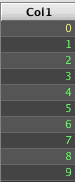
Columns can be added using the update(), updateView(), or lazyUpdate() methods:

newTable=emptyTable(10).update("Col1=i")

from deephaven import *

t1 = ttools.emptyTable(1).update("Col1 = `Hello` + ` ` + `World`")

This Deephaven statement is quite different than SQL. It creates a new table, with 10 rows, and then creates a new column by calling update(), which sets the column name equal to Col1, and the value equal to the special index value i. In a Deephaven query, i indicates the current row number of a non-ticking table as an integer. ii provides the same data, but as a long.

A sequence of statements to return a similar table in SQL Server would look similar to the following:

DECLARE @x TABLE(Col1 INT)
DECLARE @i INT
SET @i = 0
WHILE @i < 10
    BEGIN
        INSERT @x VALUES(@i)
        SET @i = @i + 1
    END

newTable

Similar to emptyTable(), newTable() can be used to create an in-memory table. The newTable() method is a bit different, in that it takes explicitly defined columns of data to add when creating the table.

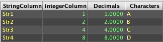
The following example starts by defining four arrays of data. These arrays are then passed into the column creation methods (col(), intCol(), doubleCol(), and charCol()), which take a name and an array of data, and create a ColumnHolder object that can be added to a table.

myStrings = ["Str1", "Str2", "Str3", "Str4"] as String[]
myInts = [1, 2, 4, 8] as int[]
myDoubles = [1.0, 2.0, 4.0, 8.0] as double[]
myCharacters = ['A', 'B', 'C', 'D'] as char[]

myTable = newTable(
        col("StringColumn", myStrings),
        intCol("IntegerColumn", myInts),
        doubleCol("Decimals", myDoubles),
        charCol("Characters" , myCharacters)
)

from deephaven import *

myStrings = ["Str1", "Str2", "Str3", "Str4"]
myInts = [1, 2, 4, 8]
myDoubles = [1.0, 2.0, 4.0, 8.0]
myCharacters = ['A', 'B', 'C', 'D']

myTable = ttools.newTable( \
    ttools.col("StringColumn", myStrings), \
    ttools.intCol("IntegerColumn", myInts), \
    ttools.doubleCol("Decimals", myDoubles), \
    ttools.charCol("Characters" , myCharacters) \
    )

readCsv

In Deephaven, readCsv() allows creating an in-memory table from a delimited text file. This is analogous to OPENROWSET() in SQL Server, or LOAD DATA in MySQL.

For example, the following is delimited text found in a file named Sample.csv:

NAME,ID
"Al Jones",123
"Tom Richards",99876

The readCsv() method can be used to create a Deephaven table as demonstrated below:

sample=readCsv("/tmp/Sample.csv")

Note: The file path from which to read the CSV file is relative to the query server.

The readCsv() method will infer appropriate types for the columns by inspecting the data being read. For instance, if all values in one of the columns will fit into long variables, long will be used for that column in the in-memory table.

Input Tables

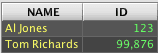
Input tables are Deephaven structures that, from the user's perspective, act more like relational database tables. On disk, they are append-only tables like other Deephaven tables. However, when used in the console, Input tables provide a table that supports CRUD operations so users can add, update, and remove data. The lastBy() method is used to provide the most recent version of a row (or the lack of a row, due to the most recent being a "delete" record).

Please refer to the following sections of the Deephaven documentation for more information:

• Creating System tables
• Creating, populating, and managing User tables
• Reading and writing data from tables, and defining tables
• Using readCsv() to read delimited text files into memory tables
• Using Input Tables

User-defined Functions

Deephaven scripts can be written in either Groovy or Python. Both support constructs for declaring user-defined functions for use within queries (closures for Groovy or functions for Python). In both cases, the return value from such a function will be a generic object that must be re-cast to the needed type for the column or expression where they will be used. These functions can also return memory tables, so both forms can be used as scalar or tabular functions.

The following examples demonstrate squaring a value in both SQL and Deephaven. This is not very useful method, but it provides a simple example of custom function.

In T-SQL, an integer squaring function can be declared as follows:

CREATE FUNCTION Square(@value AS int)
RETURNS int
BEGIN
RETURN @value * @value
END

In Deephaven, a similar function and its use are shown below.

y=emptyTable(10).update("A=i")

square={value ->
  return value * value
}

y2=y.update("B=(int)square.call(A)").ungroup()

from illumon.iris.TableTools import emptyTable
y=emptyTable(10).update("A=i")

def square(value):
  return value * value

y2=y.update("B=(int)square.call(A)").ungroup()

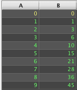
A more useful example is creating a cumulative sum function that can be applied to ticking tables in Deephaven. This example takes advantage of Deephaven's ability to flatten a table into groups of arrays using the by() method, and then re-expanding it using ungroup(). The cumulative sum function iterates each of the arrays to produce an array of sums that will then be expanded back into row data by ungroup().

x=emptyTable(10).update("A=i")
x2=x.by()

cumSum={col ->
    sum = 0;
    result = new int[col.size()];
    for (q=0;q<col.size();q++) {
        sum += col.get(q);
        result[q] = sum;
    }
    return result;
}

x2=x2.update("B=(int[])cumSum.call(A)")
x=x2.ungroup()

from illumon.iris.TableTools import emptyTable
x=emptyTable(10).update("A=i")
x2=x.by()

def cumSum(values):
  calculations = jpy.array('int', values.size())
  sum = 0
  for i in range(values.size()):
    sum += values.get(i)
    calculations[i] = sum
  return calculations

x2=x2.update("B=(int[])cumSum.call(new Object[]{A})").ungroup()

A similar result could be achieved in SQL with a correlated sub-query update:

UPDATE x
SET x1.B =(    SELECT
                 SUM(A)
               FROM x x2
               WHERE x2.A <= x1.A)
FROM x x1

However, the SQL version depends on either the data being sorted, or the addition of a row index column to use for correlation instead. In this example, the data is presorted.

In the Deephaven examples, the data from column A must be explicitly cast into an object array when being passed to the Python function, while the Groovy closure can directly accept the data in column A as-is.