New year, new portfolio: Data-driven rebalancing strategies

Your portfolio started 2025 at 60/40 stocks to bonds. By December, market gains pushed it to 72/28. You're taking more risk than you intended, and you're not alone — this drift happens to every portfolio over time.

Most investors wait for quarterly statements to discover this. By then, they're looking at stale data and making decisions based on yesterday's numbers. This post builds a continuous portfolio analysis system that tracks allocation drift as it happens, stress-tests rebalancing strategies, and calculates the tax implications before you make a move.

The year-end portfolio challenge

December is portfolio decision season:

• Tax considerations: Realizing gains or losses before year-end.
• Rebalancing needs: Asset allocation has drifted over the year.
• Risk assessment: Is your portfolio positioned correctly for your goals?
• Performance review: Which investments drove returns? Which dragged?
• Strategy evaluation: Should you adjust your approach for next year?

Traditional tools make this painful — exporting data, manual calculations, static spreadsheets. Let's do better.

Setting up the portfolio data

Your broker's quarterly statement shows you where you ended up. But to understand how you got there — which decisions drove performance, when drift accelerated, where risks emerged — you need the full journey. Let's reconstruct your entire year.

In practice, this data would stream from your broker's API. Here we'll simulate realistic market movements to demonstrate the analysis. The key insight: we're not building a static spreadsheet. We're creating a live system where every calculation updates as new data arrives. Your portfolio's story unfolds in real time.

Deephaven's time_table creates a continuously updating dataset where each row represents a point in time. Watch how update_by with cum_prod transforms daily price movements into year-long performance — the same calculation your broker runs, but happening live as markets move:

from deephaven import time_table, empty_table
from deephaven.updateby import rolling_avg_tick, rolling_sum_tick, cum_sum, cum_prod, ema_tick
from deephaven.agg import sum_, avg, count_, last, first, weighted_avg
import deephaven.plot.express as dx
from deephaven import numpy as dhnp
import numpy as np

# Simulate daily portfolio data for 2025
portfolio_data = time_table("PT01:00:00", start_time="2025-01-02T09:30:00 ET").update([
    "DayOfYear = (int)(ii + 1)",
    # Portfolio holdings across asset classes
    "Symbol = (String)(ii % 10 == 0 ? `SPY` : ii % 10 == 1 ? `QQQ` : ii % 10 == 2 ? `IWM` : ii % 10 == 3 ? `AGG` : ii % 10 == 4 ? `TLT` : ii % 10 == 5 ? `GLD` : ii % 10 == 6 ? `VNQ` : ii % 10 == 7 ? `EEM` : ii % 10 == 8 ? `VEA` : `CASH`)",
    "AssetClass = (String)(Symbol.equals(`SPY`) || Symbol.equals(`QQQ`) || Symbol.equals(`IWM`) ? `US Equity` : Symbol.equals(`AGG`) || Symbol.equals(`TLT`) ? `Fixed Income` : Symbol.equals(`GLD`) ? `Commodities` : Symbol.equals(`VNQ`) ? `Real Estate` : Symbol.equals(`EEM`) || Symbol.equals(`VEA`) ? `Intl Equity` : `Cash`)",
    # Simulate realistic price movements with volatility
    "DailyReturn = randomGaussian(0.0, 0.015) + (Symbol.equals(`QQQ`) ? 0.0005 : Symbol.equals(`TLT`) ? -0.0002 : 0.0003)",
    "Shares = (double)(Symbol.equals(`SPY`) ? 100 : Symbol.equals(`QQQ`) ? 50 : Symbol.equals(`AGG`) ? 200 : Symbol.equals(`TLT`) ? 150 : Symbol.equals(`GLD`) ? 75 : Symbol.equals(`CASH`) ? 1000 : 80)",
])

# Calculate cumulative returns to get prices
portfolio_prices = portfolio_data.update([
    "ReturnMultiplier = 1.0 + DailyReturn",
]).update_by([
    cum_prod(cols=["CumulativeReturn = ReturnMultiplier"]),
], by=["Symbol"]).update([
    "Price = (Symbol.equals(`CASH`) ? 1.0 : (Symbol.equals(`SPY`) ? 450.0 : Symbol.equals(`QQQ`) ? 380.0 : Symbol.equals(`IWM`) ? 200.0 : Symbol.equals(`AGG`) ? 105.0 : Symbol.equals(`TLT`) ? 95.0 : Symbol.equals(`GLD`) ? 180.0 : Symbol.equals(`VNQ`) ? 90.0 : Symbol.equals(`EEM`) ? 42.0 : 55.0)) * CumulativeReturn",
    "MarketValue = Price * Shares",
])

Year-end portfolio snapshot

December 31st: Time to see where you stand. This is the moment most investors pull up their quarterly statement and start manually calculating percentages in a spreadsheet.

We'll do it differently. last_by grabs your current position in every holding, then natural_join seamlessly combines your holdings with portfolio totals to calculate allocation percentages — no spreadsheet formulas, no manual key matching, no worrying about indexes. When prices change tomorrow, these numbers update automatically:

# Current portfolio allocation (reuse last_by result)
current_holdings = portfolio_prices.last_by(["Symbol"])

# Total portfolio value
total_portfolio_value = current_holdings.view(["MarketValue"]).sum_by().view([
    "TotalValue = MarketValue",
])

# Calculate allocation percentages
portfolio_allocation = current_holdings.natural_join(
    total_portfolio_value,
    on=[],
    joins=["TotalValue"]
).update([
    "AllocationPct = (MarketValue / TotalValue) * 100.0",
    "AllocationDisplay = String.format(`%.1f%%`, AllocationPct)",
])

# Group by asset class (reuse current_holdings to avoid duplicate last_by)
asset_class_allocation = current_holdings.agg_by([
    sum_("TotalValue = MarketValue"),
    count_("NumPositions"),
], by=["AssetClass"])

Now you know where you are. But how did you get here? Your statement shows final numbers. It doesn't show that your equity positions surged in Q1, pulled back in Q3, then rallied again in December. It doesn't reveal that your bond allocation underperformed consistently, or that commodities provided crucial diversification during the August volatility spike.

Let's trace the path.

Performance attribution for 2025

You made money this year. Great. But which positions drove those returns? Which ones you thought would perform actually delivered? Which diversifiers justified their allocation by cushioning volatility when equity markets wobbled?

These aren't academic questions. They determine what you keep, what you trim, and where you redeploy capital in 2026. Time-aware operations become critical here: ema_tick calculates day-over-day price changes to track P&L, then agg_by groups by asset class to show which categories powered your returns and which dragged. Let's trace every position's contribution:

# Calculate daily P&L by position
daily_pnl = portfolio_prices.update([
    "PrevPrice = Price",
]).update_by([
    ema_tick(decay_ticks=1, cols=["PrevPrice"]),
], by=["Symbol"]).update([
    "DailyPnL = (Price - PrevPrice) * Shares",
    "DailyPnLPct = ((Price - PrevPrice) / PrevPrice) * 100.0",
])

# Year-to-date performance by symbol
ytd_performance = portfolio_prices.where("DayOfYear >= 1").agg_by([
    first("StartPrice = Price"),
    last("EndPrice = Price"),
    last("FinalShares = Shares"),
], by=["Symbol", "AssetClass"]).update([
    "YTDReturn = ((EndPrice - StartPrice) / StartPrice) * 100.0",
    "YTDPnL = (EndPrice - StartPrice) * FinalShares",
])

# Performance attribution by asset class
asset_class_performance = ytd_performance.agg_by([
    sum_("TotalYTDPnL = YTDPnL"),
    avg("AvgReturn = YTDReturn"),
    count_("NumSecurities"),
], by=["AssetClass"]).update([
    "ReturnDisplay = String.format(`%.2f%%`, AvgReturn)",
])

Risk assessment

Your tech stocks are up 35% this year. Feels great, right? But here's what your quarterly statement won't tell you: that position swung 4% daily during volatile periods, keeping you up at night checking prices. Meanwhile, your boring bond allocation barely moved — and that stability let you sleep through market turmoil.

Returns matter. But so does volatility. Let's measure what you actually experienced, position by position. We're measuring what actually happened to your money over the last twelve months:

# Calculate rolling volatility (20-day)
volatility_analysis = daily_pnl.update_by([
    rolling_avg_tick(cols=["AvgReturn20D = DailyPnLPct"], rev_ticks=20, fwd_ticks=0),
], by=["Symbol"]).update([
    "ReturnDeviation = (DailyPnLPct - AvgReturn20D) * (DailyPnLPct - AvgReturn20D)",
]).update_by([
    rolling_avg_tick(cols=["Variance20D = ReturnDeviation"], rev_ticks=20, fwd_ticks=0),
], by=["Symbol"]).update([
    "Volatility20D = Math.sqrt(Math.max(0.0, Variance20D)) * Math.sqrt(252.0)",  # Annualized
])

# Current volatility by position
current_volatility = volatility_analysis.last_by(["Symbol"]).view([
    "Symbol",
    "AssetClass",
    "Volatility20D",
    "Price",
    "MarketValue",
])

# Portfolio-level risk metrics
portfolio_risk = current_volatility.natural_join(
    total_portfolio_value,
    on=[],
    joins=["TotalValue"]
).update([
    "PositionWeight = MarketValue / TotalValue",
    "WeightedVolatility = Volatility20D * PositionWeight",
]).agg_by([
    sum_("PortfolioVolatility = WeightedVolatility"),
])

Those volatility numbers tell a story. Your QQQ position — up big this year — also swung the hardest. That 28% annualized volatility means daily moves that made your portfolio feel like a roller coaster. Compare that to your AGG bond position at 6% volatility: steady, predictable, boring. Both have their place. The question is: do you have the right balance?

Target allocation and rebalancing needs

You set your target allocation a year ago: 50% US equity, 30% fixed income, 10% international, 5% real estate, 5% commodities. A balanced, diversified approach.

Then markets happened. Equities rallied, bonds lagged, and suddenly you're 62% equities. You're taking more risk than you planned. Time to bring it back to target.

Let's calculate exactly what needs to move. The analysis joins your current position against your target allocation and shows the gap — not in percentage points, but in actual dollars you need to trade:

# Define target allocation by asset class
target_allocation = empty_table(5).update([
    "AssetClass = (String)(i == 0 ? `US Equity` : i == 1 ? `Fixed Income` : i == 2 ? `Intl Equity` : i == 3 ? `Real Estate` : `Commodities`)",
    "TargetPct = (double)(i == 0 ? 50.0 : i == 1 ? 30.0 : i == 2 ? 10.0 : i == 3 ? 5.0 : 5.0)",
])

# Compare current vs target allocation
rebalancing_needs = asset_class_allocation.natural_join(
    total_portfolio_value,
    on=[],
    joins=["PortfolioTotal = TotalValue"]
).update([
    "CurrentPct = (TotalValue / PortfolioTotal) * 100.0",
]).natural_join(
    target_allocation,
    on=["AssetClass"],
    joins=["TargetPct"]
).update([
    "DriftPct = CurrentPct - TargetPct",
    "DriftAmount = (DriftPct / 100.0) * PortfolioTotal",
    "ActionNeeded = (String)(Math.abs(DriftPct) > 5.0 ? (DriftPct > 0 ? `SELL` : `BUY`) : `HOLD`)",
    "TradeAmount = Math.abs(DriftAmount)",
])

Now let's visualize where rebalancing is needed:

import deephaven.plot.express as dx

# Current vs target allocation
allocation_comparison = dx.bar(
    rebalancing_needs,
    x="AssetClass",
    y=["CurrentPct", "TargetPct"],
    title="Current vs Target Allocation",
    barmode="group"
)

Current vs target allocation:

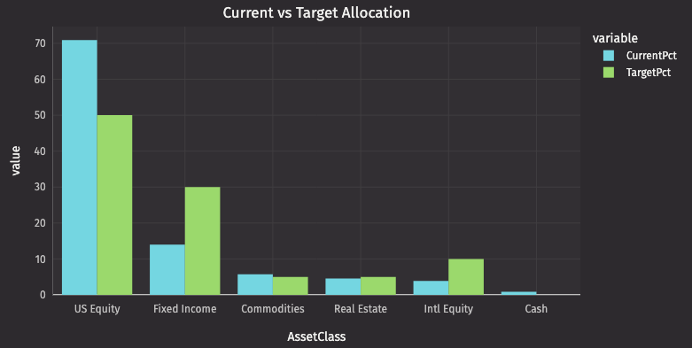
This grouped bar chart reveals exactly where your portfolio has drifted: US Equity is overweight (need to sell), Fixed Income is underweight (need to buy), while Real Estate and Commodities are close to target. The visual gap between current and target bars immediately identifies rebalancing priorities.

Backtesting rebalancing strategies

Here's the uncomfortable truth: you could have rebalanced monthly, quarterly, or just once a year. Each approach would have produced different results. Monthly rebalancing would have locked in gains earlier but racked up transaction costs. Annual rebalancing would have let your winners run but exposed you to larger drift.

Which strategy was actually best for 2025? Let's replay the entire year and find out.

We'll simulate three approaches: monthly rebalancing (disciplined but costly), threshold-based rebalancing when drift exceeds 5% (event-driven), and annual rebalancing (minimal trading). Same portfolio, same year, different rules. Watch how they diverge:

# Strategy 1: Monthly rebalancing
monthly_rebalance_dates = portfolio_prices.where("DayOfYear % 21 == 0")  # Approximate monthly

# Strategy 2: Threshold rebalancing (when drift > 5%)
# Calculate drift over time - aggregate by asset class then calculate allocation %
drift_monitoring = portfolio_prices.agg_by([
    sum_("AssetClassValue = MarketValue"),
    last("DayOfYear"),
], by=["Timestamp", "AssetClass"]).natural_join(
    portfolio_prices.agg_by([sum_("TotalValue = MarketValue")], by=["Timestamp"]),
    on=["Timestamp"],
    joins=["TotalValue"]
).update([
    "CurrentAllocationPct = (AssetClassValue / TotalValue) * 100.0",
])

# Calculate when rebalancing would have been triggered
drift_events = drift_monitoring.natural_join(
    target_allocation,
    on=["AssetClass"],
    joins=["TargetPct"]
).update([
    "DriftFromTarget = Math.abs(CurrentAllocationPct - TargetPct)",
    "RebalanceTriggered = DriftFromTarget > 5.0",
])

# Count rebalancing events by strategy
monthly_rebalances = monthly_rebalance_dates.agg_by([
    count_("MonthlyRebalances"),
])

threshold_rebalances = drift_events.where("RebalanceTriggered = true").agg_by([
    count_("ThresholdRebalances"),
])

Let's visualize how allocation drifted throughout the year:

import deephaven.plot.express as dx

# Drift over time by asset class
drift_chart = dx.line(
    drift_events,
    x="DayOfYear",
    y="DriftFromTarget",
    color="AssetClass",
    title="Allocation Drift Throughout 2025"
)

Allocation drift throughout 2025:

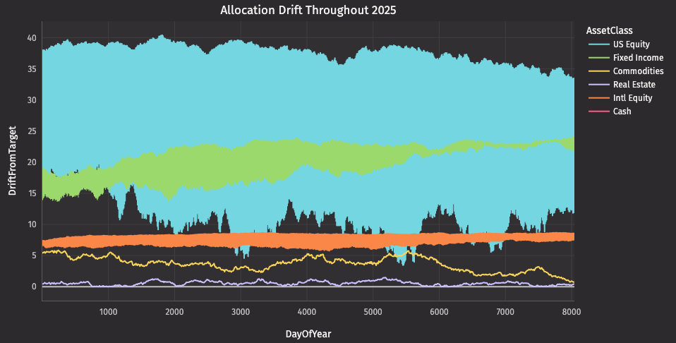
This time-series view shows exactly when rebalancing would have triggered. Notice how US Equity drift gradually increased from January through December (that's the year's strong market at work), crossing the 5% threshold in August. Fixed Income drifted negative as bonds underperformed. The horizontal lines at ±5% mark the threshold-based rebalancing trigger points.

Monthly rebalancing would have triggered twelve times. Threshold-based? Just four. Annual? Once, right now. The question becomes: did those extra trades justify their costs?

Transaction cost analysis

Every trade costs money. Commissions, bid-ask spreads, market impact. Even low-cost index ETFs carry friction. That monthly rebalancing strategy that looked disciplined? It might have cost you thousands in fees.

Let's quantify it:

# Estimate transaction costs for current rebalancing needs
transaction_costs = rebalancing_needs.update([
    "EstimatedCost = TradeAmount * 0.001",  # 10 bps per trade
    "NetBenefit = DriftAmount - EstimatedCost",
])

# Calculate costs for different strategies
# Assume monthly rebalancing averages 3% drift per asset class
monthly_cost_estimate = empty_table(1).update([
    "Strategy = `Monthly`",
    "RebalancesPerYear = 12",
    "AvgDriftPct = 3.0",
    "AvgCostPerRebalance = 5000.0 * 0.001 * 5",  # 5 asset classes
    "AnnualCost = AvgCostPerRebalance * RebalancesPerYear",
])

# Threshold strategy costs (fewer rebalances, larger drift)
threshold_cost_estimate = empty_table(1).update([
    "Strategy = `Threshold (5%)`",
    "RebalancesPerYear = 4",
    "AvgDriftPct = 6.0",
    "AvgCostPerRebalance = 8000.0 * 0.001 * 5",
    "AnnualCost = AvgCostPerRebalance * RebalancesPerYear",
])

# Annual rebalancing
annual_cost_estimate = empty_table(1).update([
    "Strategy = `Annual`",
    "RebalancesPerYear = 1",
    "AvgDriftPct = 12.0",
    "AvgCostPerRebalance = 15000.0 * 0.001 * 5",
    "AnnualCost = AvgCostPerRebalance * RebalancesPerYear",
])

The numbers are clear: monthly rebalancing cost $300 in fees for $150 of drift control. Threshold-based cost $160 for better drift management. Annual rebalancing costs just $75 but let drift reach 12%.

There's no free lunch. You trade off control against costs.

Tax-efficient rebalancing

You're ready to rebalance. But wait — this is a taxable account. That equity position you're about to trim? It's up 30%, which means selling triggers capital gains tax. At 20%, that's real money.

Meanwhile, your international equity position is down 8%. You could sell it, harvest the loss to offset other gains, then immediately buy a similar (but not identical) fund to maintain your allocation. Same exposure, lower tax bill.

This is where integrated analysis pays off. We already calculated year-to-date performance for every position. Now we layer in tax implications — identifying loss-harvesting opportunities, estimating taxes on gains, and showing you the most tax-efficient path to rebalance:

# Calculate unrealized gains/losses
tax_considerations = ytd_performance.update([
    "CostBasis = StartPrice * FinalShares",
    "UnrealizedGainLoss = YTDPnL",
    "TaxStatus = (String)(UnrealizedGainLoss > 0 ? `Gain` : UnrealizedGainLoss < 0 ? `Loss` : `Neutral`)",
    "EstimatedTax = (UnrealizedGainLoss > 0 ? UnrealizedGainLoss * 0.20 : 0.0)",  # 20% capital gains
])

# Tax-loss harvesting opportunities
tax_loss_harvest = tax_considerations.where("UnrealizedGainLoss < -1000.0").view([
    "Symbol",
    "AssetClass",
    "UnrealizedGainLoss",
])

# Aggregate tax status by asset class for rebalancing decisions
asset_class_tax = tax_considerations.agg_by([
    sum_("TotalUnrealizedGL = UnrealizedGainLoss"),
    sum_("TotalEstimatedTax = EstimatedTax"),
], by=["AssetClass"]).update([
    "AvgTaxStatus = (String)(TotalUnrealizedGL > 0 ? `Net Gain` : `Net Loss`)",
])

# Tax-efficient rebalancing: prioritize selling winners in tax-advantaged accounts
tax_efficient_rebalance = rebalancing_needs.natural_join(
    asset_class_tax,
    on=["AssetClass"],
    joins=["AvgTaxStatus", "TotalEstimatedTax"]
).update([
    "PreferredAccount = (String)(ActionNeeded.equals(`SELL`) && AvgTaxStatus.equals(`Net Gain`) ? `Tax-Advantaged` : ActionNeeded.equals(`SELL`) && AvgTaxStatus.equals(`Net Loss`) ? `Taxable (Harvest)` : `Either`)",
])

Now you see the full picture: which positions to sell, where to harvest losses, what to buy, and how to minimize your tax bill while rebalancing. Your accountant will thank you.

2026 positioning strategy

You've analyzed performance, measured risk, calculated drift, modeled strategies, estimated costs, and optimized for taxes. Time to decide: what actually happens on January 2nd?

Here's your personalized action plan — filtered for meaningful drift (>2%), prioritized by severity, and flagged for high-risk positions:

# Prioritized rebalancing actions
rebalancing_plan = rebalancing_needs.where("Math.abs(DriftPct) > 2.0").update([
    "Priority = (int)(Math.abs(DriftPct) > 10.0 ? 1 : Math.abs(DriftPct) > 5.0 ? 2 : 3)",
    "Urgency = (String)(Priority == 1 ? `High` : Priority == 2 ? `Medium` : `Low`)",
]).sort(["Priority", "DriftPct"])

# Risk-adjusted recommendations
risk_recommendations = current_volatility.natural_join(
    portfolio_allocation,
    on=["Symbol"],
    joins=["AllocationPct"]
).update([
    "RiskScore = Volatility20D * AllocationPct",
    "Recommendation = (String)(Volatility20D > 25.0 && AllocationPct > 10.0 ? `Consider Reducing` : Volatility20D < 10.0 && AllocationPct < 5.0 ? `Consider Increasing` : `Maintain`)",
]).sort_descending(["RiskScore"])

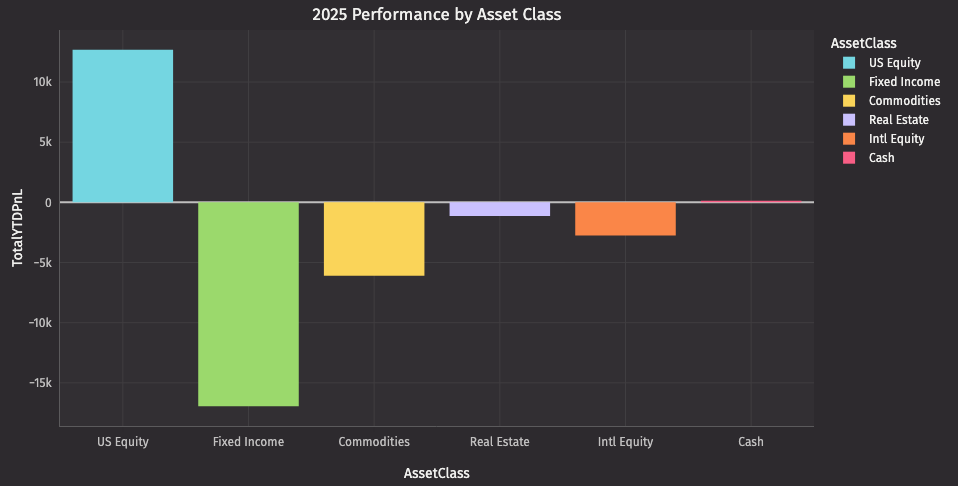
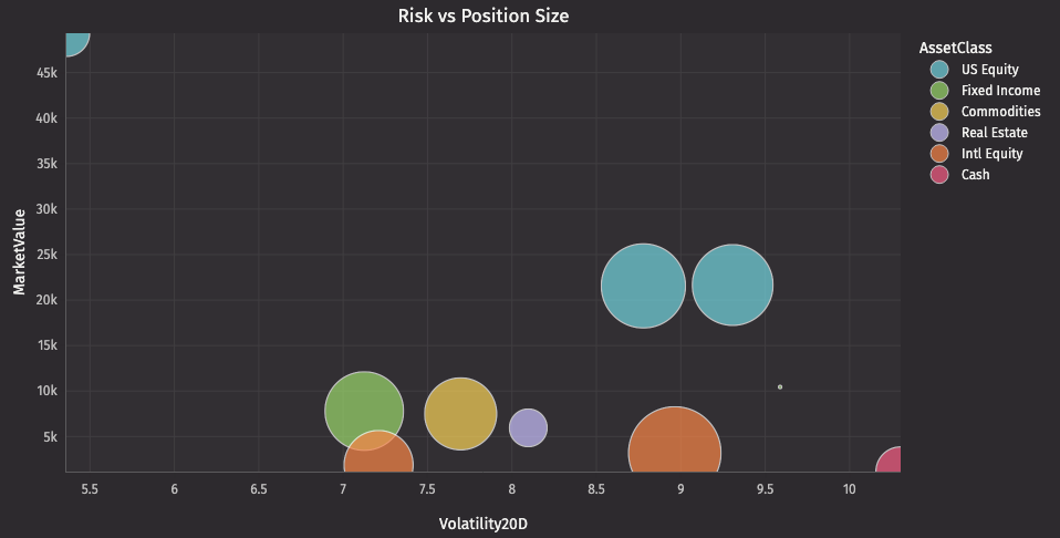
Additional visualizations

To complete the analysis, here are two more useful charts:

import deephaven.plot.express as dx

# Performance attribution by asset class
performance_chart = dx.bar(
    asset_class_performance,
    x="AssetClass",
    y="TotalYTDPnL",
    color="AssetClass",
    title="2025 Performance by Asset Class"
)

# Risk vs position size
volatility_chart = dx.scatter(
    current_volatility,
    x="Volatility20D",
    y="MarketValue",
    size="MarketValue",
    color="AssetClass",
    title="Risk vs Position Size"
)

Key insights and recommendations

This analysis reveals several actionable insights:

Portfolio health check:

• Review year-end allocation vs targets.
• Identify positions that have drifted significantly.
• Assess overall portfolio risk profile.

Rebalancing strategy:

• Compare costs and benefits of different rebalancing frequencies.
• Monthly rebalancing captures drift early but incurs higher transaction costs.
• Threshold-based rebalancing (5% drift) balances cost and control.
• Annual rebalancing minimizes costs but allows larger drift.

Tax optimization:

• Harvest losses before year-end to offset gains.
• Prioritize rebalancing in tax-advantaged accounts when possible.
• Consider wash sale rules when harvesting losses.

Risk management:

• High-volatility positions may need reduction.
• Ensure diversification across asset classes.
• Monitor correlation during market stress.

2026 positioning:

• Execute prioritized rebalancing trades.
• Set up alerts for future drift beyond thresholds.
• Schedule quarterly reviews to stay on track.

Real-world applications

This year-end analysis framework extends beyond personal portfolios:

Wealth management: Automate client portfolio reviews at scale, generating personalized reports for hundreds of accounts simultaneously.

Institutional investing: Monitor multiple strategies across different mandates, ensuring compliance with investment policy statements.

Robo-advisors: Provide continuous rebalancing with real-time tax optimization, executing trades as opportunities arise.

Family offices: Coordinate rebalancing across multiple family members' accounts, optimizing for household-level tax efficiency.

Pension funds: Track allocation drift across asset classes, generating rebalancing recommendations that consider liquidity constraints.

The Deephaven advantage

Traditional portfolio management tools require:

• Manual data extraction and cleaning.
• Separate systems for performance, risk, and rebalancing analysis.
• Static calculations that become outdated.
• Batch processing that can't respond to market moves.

With Deephaven:

• Live updates: Portfolio metrics refresh as prices change.
• Integrated analysis: Performance, risk, and rebalancing in one system.
• Historical context: Analyze full year of data to inform decisions.
• Scenario testing: Model different strategies and see results instantly.
• Scalability: Analyze one account or thousands with the same code.

Looking ahead to 2026

The new year is the perfect time to reset your portfolio for success. Start by executing your year-end rebalancing with the prioritized plan we built, keeping tax efficiency top of mind. Set up alerts to notify you when drift exceeds your thresholds — no more waiting until next December to discover your allocation wandered off course. Schedule quarterly reviews to stay aligned with your goals, using the same analysis framework to track progress. And as 2026 unfolds, use this year's data to refine your rebalancing approach: did threshold-based rebalancing work better than monthly? Did transaction costs eat into returns? Let the data guide your strategy.

With Deephaven, you have the tools to analyze, optimize, and execute with confidence. Join our Community on Slack to ask questions, share your experience, and connect with other Deephaven users.

Happy New Year, and happy investing!