Deephaven is now available in R!

Deephaven's powerful real-time analytics engine makes an invaluable addition to any data scientist's toolkit. Up to this point, it has been available through Python, Groovy, Java, Javascript, C++, and Go. However, many data scientists spend their days in R, due to its extensive ecosystem of tools for data science and statistical analysis. For the first time, Deephaven Community Core has a client available as an R package!

The new Deephaven R client bridges the gap between Deephaven's performance and scalability and R's extensive suite of data science and statistical analysis tools. In this blog post, we will demonstrate the usage of the Deephaven R client by generating real-time data and training a regression model in R. As the data stream updates, the model parameters and corresponding plots dynamically evolve.

Unlock real-time data analysis with ease in R.

A performance-first model

R is a major player in the data science game for a reason. If you can think of a problem in modern statistics or machine learning, there's probably at least one R package to handle it. It's easy to learn for newcomers and is my preferred package for data visualization (ggplot2 is my all-time favorite plotting API). However, R never claimed to be the fastest car in the race - it simply wasn't built for remarkable performance, smooth handling of massive (>10M rows) datasets, or live time-series data. That's where Deephaven comes in. Deephaven makes working with massive real-time datasets a breeze, providing intuitive SQL-like table operations with unparalleled performance. With the new R client, you can combine the greatest strengths of R and Deephaven into a true data science powerhouse. Let's dive in and see what you can do with the R client today with an example of polynomial regression on a real-time dynamic dataset.

Real-time regression

To follow along, you'll need to install the Deephaven R client. The source code and installation instructions can be found in the GitHub repo's README. The current client must be built from source. While the RStudio IDE is recommended for this tutorial, you can use any appropriate IDE.

First, we’re going to need a running Deephaven server. We'll assume that your server is running on localhost:10000 for the remainder of this post. Then, fire up an R IDE and import the Deephaven client, called rdeephaven, as well as ggplot2 for plots.

library(rdeephaven)
library(ggplot2)

To connect to a running Deephaven server, use the ClientOptions class to specify authentication details and the Client class to establish your connection.

# this automatically defaults to default authentication
client_options <- ClientOptions$new()
client <- Client$new(target="localhost:10000", client_options=client_options)

tip

Once the client is installed, you can view documentation with the typical ? operator. You might read up on the building blocks of our API with ?Client, ?TableHandle, and ?ClientOptions.

Now, client is our gateway to the Deephaven server. We can use it to retrieve references to tables already on the server, to import new tables to the server, and to run scripts.

We're going to use Deephaven to generate noisy data from a cubic polynomial. Navigate to the Deephaven IDE at localhost:10000 and run the following code.

import os
os.system("pip install scipy")

from deephaven import time_table
import scipy.stats as sts

domain = sts.uniform(loc=-3, scale=4)
def my_polynomial(x):
    return x**3 + 3*(x**2) - 2 + sts.norm(loc=0, scale=1).rvs()

data_table = time_table("PT00:00:2.00").\
    update(["x = (float)domain.rvs()", "y = (float)my_polynomial(x)"]).\
    drop_columns(["Timestamp"])

Every 2 seconds, we draw a random point $x_0$ between $-3$ and $1$ and evaluate $y = x_0^3 + 3x_0^2 - 2 + \epsilon$, where $\epsilon \sim \mathcal{N}(0, 1)$:

We can use the data generated here to reverse-engineer the coefficients from the original data-generating function. This is done with a statistical technique called regression. Since we know that the data come from a polynomial, we will use a regression variant called polynomial regression. R makes regression easier than any language I've ever used - just a single line of code! So, let's use the R client to perform a regression analysis on the dynamic data that Deephaven is generating. Navigate to your R session and pull a reference to the ticking table of interest.

data_table <- client$open_table("data_table")

We can now use data_table to convert the ticking table on the server to an R Data Frame via data_table$to_data_frame(). Since data frames are static objects, the data frame cannot tick with the table on the server. However, data_table does keep track of server-side updates, so every time you call data_table$to_data_frame(), you will get a data frame of the most recent data from the server. Let's use this to train a polynomial regression model.

current_data_frame <- data_table$to_data_frame()
model <- lm(y ~ x + I(x^2) + I(x^3), data=current_data_frame)

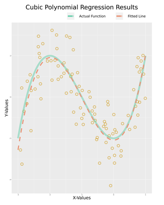
Now, we use ggplot2 to plot the data-generating function, the line of best fit according to our regression model, and the actual data in our table.

cubic_polynomial <- function(x, a, b, c, d) {
    return(a*(x^3) + b*(x^2) + c*x + d)
}

regression_plot <- ggplot() +
    xlim(-3, 1) +
    geom_point(aes(x = current_data_frame$x, y = current_data_frame$y),
        size = 5, shape = 1, stroke = 3, color = "darkgoldenrod3", alpha = 0.5) +
    geom_function(fun = cubic_polynomial, args = list(a = 1, b = 3, c = 0, d = -2),
        aes(color = "Actual Function     "), linewidth = 5, alpha = 0.5) +
    geom_function(fun = cubic_polynomial, args = list(
            a = model$coefficients[[4]], b = model$coefficients[[3]],
            c = model$coefficients[[2]], d = model$coefficients[[1]]),
        aes(color = "Fitted Line     "), linewidth = 3, linetype = "dashed") +
    labs(x = "X-Values", y = "Y-Values") +
    ggtitle("Cubic Polynomial Regression Results") +
    scale_colour_manual(name="",
        values=c("Actual Function     " = "aquamarine3",
                    "Fitted Line     " = "darksalmon")) +
    theme(plot.title = element_text(size = 36, hjust = 0.25),
        axis.title = element_text(size = 25),
        legend.text = element_text(size=20),
        legend.position = "top",
        legend.justification = "right",
        legend.spacing.x = unit(1, 'cm'),
        legend.key.size = unit(1.5, "cm"),
        plot.margin = margin(1, 2.5, 1, 1, "cm"))

regression_plot

Depending on how much data you have in your table when this code is run, you'll see something like this:

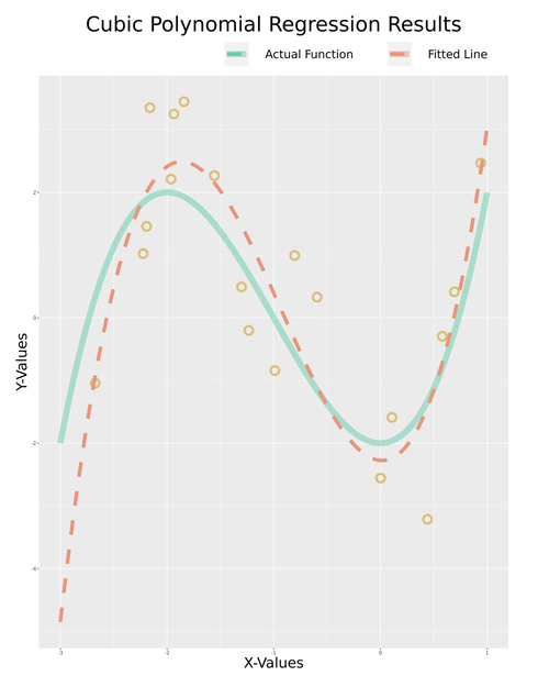
From the plot, you can see that the model matches the data-generating function pretty well. However, if you run the previous two code blocks again, you'll see that your model has gotten better. This is because the table on the server is dynamic, and more data has poured in since the model was initially trained.

This is how the Deephaven R client gives R new superpowers - Deephaven enables your vanilla R code to capture new data and all the resulting model improvements without needing any additional infrastructure for handling the real-time case.

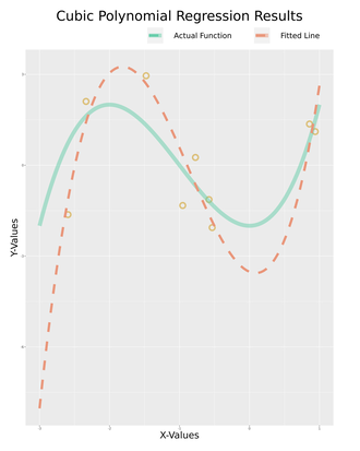
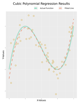
To make this crystal clear, we'll wrap the previous code blocks up into a function and call it 3 times, each time waiting for 80 seconds until the next call to exaggerate the differences between plots. You'll see that every time the plot is made, we have more data, and the model fit is a little better. The difference will be most obvious if you also restart the ticking Deephaven table in the IDE.

plot_cubic_regression <- function(table_handle) {

    # convert table handle to dataframe
    current_data_frame <- table_handle$to_data_frame()
    # run cubic polynomial regression
    model <- lm(y ~ x + I(x^2) + I(x^3), data=current_data_frame)

    # plot the results
    regression_plot <- ggplot() +
        xlim(-3, 1) +
        geom_point(aes(x = current_data_frame$x, y = current_data_frame$y),
            size = 5, shape = 1, stroke = 3, color = "darkgoldenrod3", alpha = 0.5) +
        geom_function(fun = cubic_polynomial, args = list(a = 1, b = 3, c = 0, d = -2),
            aes(color = "Actual Function     "), linewidth = 5, alpha = 0.5) +
        geom_function(fun = cubic_polynomial, args = list(
                a = model$coefficients[[4]], b = model$coefficients[[3]],
                c = model$coefficients[[2]], d = model$coefficients[[1]]),
            aes(color = "Fitted Line     "), linewidth = 3, linetype = "dashed") +
        labs(x = "X-Values", y = "Y-Values") +
        ggtitle("Cubic Polynomial Regression Results") +
        scale_colour_manual(name="",
            values=c("Actual Function     " = "aquamarine3",
                     "Fitted Line     " = "darksalmon")) +
        theme(plot.title = element_text(size = 36, hjust = 0.25),
            axis.title = element_text(size = 25),
            legend.text = element_text(size=20),
            legend.position = "top",
            legend.justification = "right",
            legend.spacing.x = unit(1, 'cm'),
            legend.key.size = unit(1.5, "cm"),
            plot.margin = margin(1, 2.5, 1, 1, "cm"))

    return(regression_plot)
}

plot_cubic_regression(sample_table)
Sys.sleep(80)
plot_cubic_regression(sample_table)
Sys.sleep(80)
plot_cubic_regression(sample_table)

Now, that's certainly not something you can do in R alone. In fact, it's the easiest way I've found to pull real-time data into R and work with it comfortably. If you have models that need to be updated regularly, and your data comes from Kafka streams, a REST API, Deephaven itself, or any other updating source, the Deephaven R client will be the easiest real-time data solution in R for you, too.

Where is the R client going?

In this first release, the R client is equipped with the basic functionality required of a client. However, our roadmap includes many interesting and useful features. Here are some of my favorites:

• Using Deephaven table operations from R in a familiar, tidyverse-style API.
• Constructing new static and ticking Deephaven tables from within the R client.
• Construct Deephaven queries directly using R code.
• Easy install from CRAN via install.packages("rdeephaven").
• Support for MacOS and Windows.

As we build out new features for the R client, the kinds of awesome use cases we can display will grow and grow. However, even in its current state, it solves problems that R has no hope of solving on its own.

Useful resources

If you're interested in anything you've read today, head to deephaven.io to learn more about Deephaven, or check out the user guide to get started with Deephaven Community Core. For more information about the R client, we currently have inline documentation available, accessible via ? in R. Full documentation pages are coming soon. If you have any other questions or want to share an interesting use case, feel free to contact us on the Community Slack channel!

Wrapping up

The new Deephaven R client is a powerful tool for any data scientist. As the client matures, so will its capabilities and ease of use as the way of working with snapshots of real-time data in R. From constructing regression models and making plots as we did here, to triggering queries from data updates, to creating beautiful R webapps backed with ticking data, the possibilities are endless. We trust that you can find amazing use cases for this tool, and it's only just getting started.