Building real-time trading dashboards with Deephaven | Blog

In financial trading, milliseconds matter. Traditional data processing tools often struggle to keep up with modern markets, where thousands of trades per second generate massive streams of data that need to be processed, analyzed, and visualized in real-time.

In this post, we'll build a comprehensive real-time trading dashboard using Deephaven, demonstrating its table-oriented approach to financial data processing.

Build a production-grade trading dashboard with live P&L, risk monitoring, and technical analysis in 100 lines of Python. Everything updates automatically as market data flows in—no polling, no event handlers, no complexity.

The challenge of real-time trading data

Modern trading systems face several critical challenges:

Volume: Markets generate millions of data points per second.
Latency: Decisions must be made in microseconds to milliseconds.
Complexity: Multiple data sources need to be correlated and analyzed simultaneously.
Reliability: System failures can result in significant financial losses.

Traditional approaches often require complex architectures with multiple systems that handle ingestion, processing, storage, and visualization separately. Deephaven provides a unified platform where all these operations happen in a single environment.

Setting up our real-time trading environment

Let's start by creating a simulated real-time market data feed and building our dashboard step by step.

Simulating market data

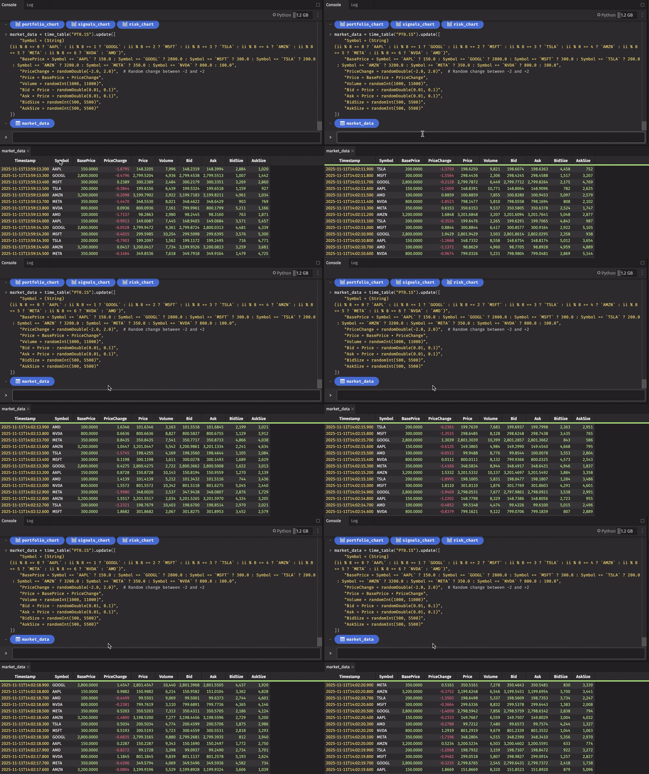
First, we'll create a realistic market data simulator that generates ticking data for multiple symbols:

from deephaven import time_table

# Create a time table that ticks every 100ms
market_data = time_table("PT0.1S").update([
    "Symbol = (String)(ii % 8 == 0 ? `AAPL` : ii % 8 == 1 ? `GOOGL` : ii % 8 == 2 ? `MSFT` : ii % 8 == 3 ? `TSLA` : ii % 8 == 4 ? `AMZN` : ii % 8 == 5 ? `META` : ii % 8 == 6 ? `NVDA` : `AMD`)",
    "BasePrice = Symbol == `AAPL` ? 150.0 : Symbol == `GOOGL` ? 2800.0 : Symbol == `MSFT` ? 300.0 : Symbol == `TSLA` ? 200.0 : Symbol == `AMZN` ? 3200.0 : Symbol == `META` ? 350.0 : Symbol == `NVDA` ? 800.0 : 100.0",
    "PriceChange = randomDouble(-2.0, 2.0)",  # Random change between -2 and +2
    "Price = BasePrice + PriceChange",
    "Volume = randomInt(1000, 11000)",
    "Bid = Price - randomDouble(0.01, 0.1)",
    "Ask = Price + randomDouble(0.01, 0.1)",
    "BidSize = randomInt(500, 5500)",
    "AskSize = randomInt(500, 5500)"
])

Real-time price calculations

Now let's add some sophisticated real-time calculations that traders typically need:

from deephaven.updateby import rolling_avg_tick, rolling_std_tick, ema_tick, rolling_sum_tick, delta

# First add calculated columns, then apply rolling operations
market_data_with_calcs = market_data.update([
    "DollarsTraded = Price * Volume"
])

# Calculate real-time moving averages and technical indicators
enriched_data = market_data_with_calcs.update_by(ops=[
    # 20-period simple moving average
    rolling_avg_tick(cols=["SMA_20 = Price"], rev_ticks=20, fwd_ticks=0),
    # 50-period simple moving average
    rolling_avg_tick(cols=["SMA_50 = Price"], rev_ticks=50, fwd_ticks=0),
    # Exponential moving average with 10-tick decay
    ema_tick(decay_ticks=10, cols=["EMA = Price"]),
    # Rolling standard deviation for volatility
    rolling_std_tick(cols=["Volatility = Price"], rev_ticks=20, fwd_ticks=0),
    # Volume-weighted average price over last 100 ticks
    rolling_sum_tick(cols=["DollarsTradedSum = DollarsTraded", "VolumeSum = Volume"], rev_ticks=100, fwd_ticks=0)
], by=["Symbol"]).update([
    # VWAP calculation
    "VWAP = DollarsTradedSum / VolumeSum"
])

# Add price change calculations using delta operation
enriched_data_with_changes = enriched_data.update_by(ops=[
    # Calculate price change from previous row
    delta(cols=["PriceChange = Price"])
], by=["Symbol"]).update([
    # Percentage change calculation
    "PctChange = isNull(PriceChange) ? 0.0 : PriceChange / (Price - PriceChange) * 100.0"
])

# Add trading signals
trading_signals = enriched_data_with_changes.update([
    "BullishSignal = SMA_20 > SMA_50 && Price > EMA",
    "BearishSignal = SMA_20 < SMA_50 && Price < EMA",
    "HighVolatility = Volatility > 0.25",
    "Signal = BullishSignal ? `BUY` : BearishSignal ? `SELL` : `HOLD`"
])

Real-time portfolio tracking

Let's create a portfolio that tracks our positions and P&L in real-time:

from deephaven import new_table, agg
from deephaven.column import string_col, int_col, double_col

# Define initial portfolio positions
# In a real system, this would be loaded from a database or position management system
portfolio_positions = new_table([
    string_col("Symbol", ["AAPL", "GOOGL", "MSFT", "TSLA", "AMZN", "META", "NVDA", "AMD"]),
    int_col("Shares", [500, 100, 750, 300, 150, 400, 250, 800]),
    double_col("AvgCost", [148.0, 2750.0, 295.0, 195.0, 3150.0, 340.0, 780.0, 95.0])
])

# Join with current market prices to calculate real-time P&L
# We only need Price from market_data, so we'll select just what we need
current_prices = market_data.last_by("Symbol").view(["Symbol", "Price"])

portfolio_pnl = portfolio_positions.natural_join(
    current_prices,
    on=["Symbol"]
).update([
    "CurrentValue = Shares * Price",
    "CostBasis = Shares * AvgCost",
    "UnrealizedPnL = CurrentValue - CostBasis",
    "PnLPercent = (UnrealizedPnL / CostBasis) * 100.0",
    "PnLPerShare = Price - AvgCost"
])

# Calculate portfolio-level aggregations
portfolio_summary = portfolio_pnl.agg_by(aggs=[
    agg.sum_(["TotalValue = CurrentValue", "TotalCost = CostBasis", "TotalPnL = UnrealizedPnL"])
]).update([
    "TotalPnLPercent = (TotalPnL / TotalCost) * 100.0"
])

Advanced real-time analytics

Risk monitoring

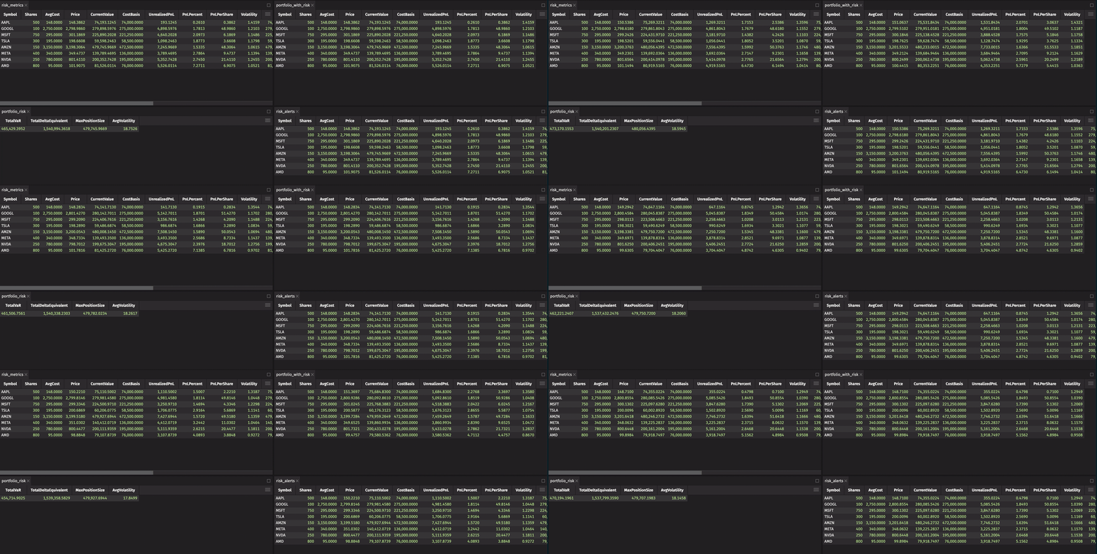
Real-time risk monitoring is crucial for any trading operation. Let's implement some key risk metrics:

from deephaven import agg

# Join portfolio with volatility data from trading signals
portfolio_with_risk = portfolio_pnl.natural_join(
    trading_signals.last_by("Symbol").view(["Symbol", "Volatility"]),
    on=["Symbol"]
)

# Calculate real-time risk metrics
risk_metrics = portfolio_with_risk.update([
    "PositionSize = abs(CurrentValue)",
    "Volatility20D = Volatility * 15.87",  # Annualized volatility (sqrt(252) ≈ 15.87)
    "VaR_95 = PositionSize * 1.65 * Volatility20D / 100.0",  # 95% Value at Risk
    "Beta = 1.0",  # Simplified - in practice, calculate vs market index
    "DeltaEquivalent = Shares * Price * Beta",
    "HighVolatility = Volatility > 0.25"
])

# Portfolio-level risk aggregation
portfolio_risk = risk_metrics.agg_by(aggs=[
    agg.sum_(["TotalVaR = VaR_95", "TotalDeltaEquivalent = DeltaEquivalent"]),
    agg.max_("MaxPositionSize = PositionSize"),
    agg.avg("AvgVolatility = Volatility20D")
])

# Risk alerts for positions exceeding thresholds
risk_alerts = risk_metrics.where([
    "VaR_95 > 50000 || abs(PnLPercent) > 10.0 || HighVolatility"
]).update([
    "AlertType = VaR_95 > 50000 ? `HIGH_VAR` : abs(PnLPercent) > 10.0 ? `LARGE_PNL` : `HIGH_VOLATILITY`",
    "AlertMessage = `Risk Alert: ` + AlertType + ` for ` + Symbol"
])

Market microstructure analysis

Let's analyze the bid-ask spread and market depth:

from deephaven.updateby import rolling_avg_tick, rolling_std_tick

# Bid-ask spread analysis using our real-time market data
spread_analysis = market_data.update([
    "Spread = Ask - Bid",
    "SpreadBps = Spread / ((Bid + Ask) / 2.0) * 10000",  # Spread in basis points
    "MidPrice = (Bid + Ask) / 2.0",
    "ImbalanceRatio = BidSize / (BidSize + AskSize)",
    "TotalDepth = BidSize + AskSize"
]).update_by(ops=[
    rolling_avg_tick(cols=["AvgSpreadBps = SpreadBps"], rev_ticks=50, fwd_ticks=0),
    rolling_std_tick(cols=["SpreadVolatility = SpreadBps"], rev_ticks=50, fwd_ticks=0)
], by=["Symbol"])

# Market quality metrics
market_quality = spread_analysis.last_by("Symbol").update([
    "LiquidityScore = TotalDepth / AvgSpreadBps",
    "MarketQuality = LiquidityScore > 1000 ? `EXCELLENT` : LiquidityScore > 500 ? `GOOD` : LiquidityScore > 100 ? `FAIR` : `POOR`"
])

Real-time alerts and notifications

# Price movement alerts using our real-time trading signals
price_alerts = trading_signals.where([
    "abs(PctChange) > 2.0 || Volume > 8000"
]).update([
    "AlertType = abs(PctChange) > 5.0 ? `MAJOR_MOVE` : abs(PctChange) > 2.0 ? `SIGNIFICANT_MOVE` : `HIGH_VOLUME`",
    "Direction = PctChange > 0 ? `UP` : `DOWN`",
    "AlertMessage = Symbol + ` ` + AlertType + ` ` + Direction + `: ` + PctChange + `% on volume ` + Volume"
])

Price Alerts

Bringing it all together: The real-time dashboard

Now that we've built all the components, let's see how they work together. All these tables update automatically as market data flows in - portfolio P&L, risk metrics, alerts, and market quality all refresh in real-time without any additional code.

Your live dashboard includes:

trading_signals: Real-time prices with technical indicators (SMA, EMA, VWAP) and buy/sell signals
portfolio_pnl: Current position values and unrealized P&L updating with every price tick
portfolio_summary: Aggregate portfolio metrics showing total value and return
risk_metrics: Position-level risk calculations including VaR and volatility measures
risk_alerts: Filtered view showing only positions that breach risk thresholds
spread_analysis: Market microstructure data with bid-ask spreads and depth
price_alerts: Significant price movements and high-volume events as they happen

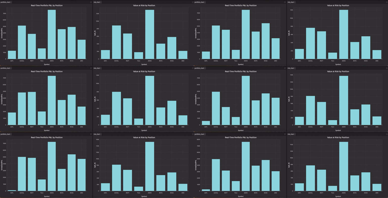
Each table updates automatically as new market data arrives. Open any table in the Deephaven UI to see live updates, sort, filter, or create custom visualizations. You can also use Deephaven's plotting capabilities to visualize this data:

import deephaven.plot.express as dx

# Visualize portfolio performance
portfolio_chart = dx.bar(portfolio_pnl, x="Symbol", y="UnrealizedPnL",
                          title="Real-Time Portfolio P&L by Position")

# Track technical indicators
signals_chart = dx.line(trading_signals.where("Symbol = `AAPL`"),
                        x="Timestamp", y=["Price", "SMA_20", "SMA_50"],
                        title="AAPL Price with Moving Averages")

# Monitor risk exposure
risk_chart = dx.bar(risk_metrics, x="Symbol", y="VaR_95",
                    title="Value at Risk by Position")

Bar Chart Signal Chart

All visualizations update in real-time as the underlying tables change - no polling, no manual refreshes, no complex event handlers.

How the architecture works

A few characteristics of the table-oriented approach are worth noting:

Unified operations: Data ingestion, processing, and visualization all work with the same table abstraction. There's no separate system for streaming versus batch, or for analytics versus visualization.

Automatic propagation: When market_data updates, all dependent tables (trading_signals, portfolio_pnl, risk_metrics) update automatically. You define the relationships once, and Deephaven handles the update propagation.

Incremental updates: Only changed data gets reprocessed. When a single price ticks, Deephaven recalculates only the affected rows in dependent tables, not the entire dataset.

Columnar storage: Tables use columnar storage internally, which is efficient for both memory usage and analytical queries on large datasets.

These properties make the platform well-suited for high-frequency data processing where both latency and throughput matter.

Performance considerations for production

When deploying this dashboard to production trading systems, consider these optimization strategies:

Data retention: For high-frequency data, implement retention policies to keep memory usage manageable:

# Keep only the last hour of tick data
recent_market_data = market_data.where("Timestamp >= now() - 'PT1H'")

Selective updates: For computationally expensive indicators, sample at lower frequencies:

# Update slow indicators every 10 ticks instead of every tick
slow_indicators = market_data.where("ii % 10 == 0").update_by(ops=[...])

Partitioned tables: For historical data storage, partition by symbol for efficient queries:

historical_trades = market_data.partition_by("Symbol")

Selective subscriptions: Only subscribe to the specific tables and columns your UI needs, rather than the entire dashboard. This reduces network overhead and browser memory usage.

Deephaven's incremental computation engine ensures that only changed data is reprocessed, making these strategies highly effective even with thousands of updates per second.

Complete code example

For your convenience, here's the complete working code for building a real-time trading dashboard with Deephaven:

Complete Real-Time Trading Dashboard Code

# =============================================================================
# Imports
# =============================================================================
from deephaven import time_table, new_table, agg
from deephaven.updateby import rolling_avg_tick, rolling_std_tick, ema_tick, rolling_sum_tick, delta
from deephaven.column import string_col, int_col, double_col

# =============================================================================
# Market Data Simulation
# =============================================================================
# Create a time table that ticks every 100ms
market_data = time_table("PT0.1S").update([
    "Symbol = (String)(ii % 8 == 0 ? `AAPL` : ii % 8 == 1 ? `GOOGL` : ii % 8 == 2 ? `MSFT` : ii % 8 == 3 ? `TSLA` : ii % 8 == 4 ? `AMZN` : ii % 8 == 5 ? `META` : ii % 8 == 6 ? `NVDA` : `AMD`)",
    "BasePrice = Symbol == `AAPL` ? 150.0 : Symbol == `GOOGL` ? 2800.0 : Symbol == `MSFT` ? 300.0 : Symbol == `TSLA` ? 200.0 : Symbol == `AMZN` ? 3200.0 : Symbol == `META` ? 350.0 : Symbol == `NVDA` ? 800.0 : 100.0",
    "PriceChange = randomDouble(-2.0, 2.0)",  # Random change between -2 and +2
    "Price = BasePrice + PriceChange",
    "Volume = randomInt(1000, 11000)",
    "Bid = Price - randomDouble(0.01, 0.1)",
    "Ask = Price + randomDouble(0.01, 0.1)",
    "BidSize = randomInt(500, 5500)",
    "AskSize = randomInt(500, 5500)"
])

# =============================================================================
# Technical Indicators
# =============================================================================
# First add calculated columns, then apply rolling operations
market_data_with_calcs = market_data.update([
    "DollarsTraded = Price * Volume"
])

# Calculate real-time moving averages and technical indicators
enriched_data = market_data_with_calcs.update_by(ops=[
    # 20-period simple moving average
    rolling_avg_tick(cols=["SMA_20 = Price"], rev_ticks=20, fwd_ticks=0),
    # 50-period simple moving average
    rolling_avg_tick(cols=["SMA_50 = Price"], rev_ticks=50, fwd_ticks=0),
    # Exponential moving average with 10-tick decay
    ema_tick(decay_ticks=10, cols=["EMA = Price"]),
    # Rolling standard deviation for volatility
    rolling_std_tick(cols=["Volatility = Price"], rev_ticks=20, fwd_ticks=0),
    # Volume-weighted average price over last 100 ticks
    rolling_sum_tick(cols=["DollarsTradedSum = DollarsTraded", "VolumeSum = Volume"], rev_ticks=100, fwd_ticks=0)
], by=["Symbol"]).update([
    # VWAP calculation
    "VWAP = DollarsTradedSum / VolumeSum"
])

# Add price change calculations using delta operation
enriched_data_with_changes = enriched_data.update_by(ops=[
    # Calculate price change from previous row
    delta(cols=["PriceChange = Price"])
], by=["Symbol"]).update([
    # Percentage change calculation
    "PctChange = isNull(PriceChange) ? 0.0 : PriceChange / (Price - PriceChange) * 100.0"
])

# Add trading signals
trading_signals = enriched_data_with_changes.update([
    "BullishSignal = SMA_20 > SMA_50 && Price > EMA",
    "BearishSignal = SMA_20 < SMA_50 && Price < EMA",
    "HighVolatility = Volatility > 0.25",
    "Signal = BullishSignal ? `BUY` : BearishSignal ? `SELL` : `HOLD`"
])

# =============================================================================
# Portfolio Tracking
# =============================================================================
# Define initial portfolio positions
# In a real system, this would be loaded from a database or position management system
portfolio_positions = new_table([
    string_col("Symbol", ["AAPL", "GOOGL", "MSFT", "TSLA", "AMZN", "META", "NVDA", "AMD"]),
    int_col("Shares", [500, 100, 750, 300, 150, 400, 250, 800]),
    double_col("AvgCost", [148.0, 2750.0, 295.0, 195.0, 3150.0, 340.0, 780.0, 95.0])
])

# Join with current market prices to calculate real-time P&L
# We only need Price from market_data, so we'll select just what we need
current_prices = market_data.last_by("Symbol").view(["Symbol", "Price"])

portfolio_pnl = portfolio_positions.natural_join(
    current_prices,
    on=["Symbol"]
).update([
    "CurrentValue = Shares * Price",
    "CostBasis = Shares * AvgCost",
    "UnrealizedPnL = CurrentValue - CostBasis",
    "PnLPercent = (UnrealizedPnL / CostBasis) * 100.0",
    "PnLPerShare = Price - AvgCost"
])

# Calculate portfolio-level aggregations
portfolio_summary = portfolio_pnl.agg_by(aggs=[
    agg.sum_(["TotalValue = CurrentValue", "TotalCost = CostBasis", "TotalPnL = UnrealizedPnL"])
]).update([
    "TotalPnLPercent = (TotalPnL / TotalCost) * 100.0"
])

# =============================================================================
# Risk Monitoring
# =============================================================================
# Join portfolio with volatility data from trading signals
portfolio_with_risk = portfolio_pnl.natural_join(
    trading_signals.last_by("Symbol").view(["Symbol", "Volatility"]),
    on=["Symbol"]
)

# Calculate real-time risk metrics
risk_metrics = portfolio_with_risk.update([
    "PositionSize = abs(CurrentValue)",
    "Volatility20D = Volatility * 15.87",  # Annualized volatility (sqrt(252) ≈ 15.87)
    "VaR_95 = PositionSize * 1.65 * Volatility20D / 100.0",  # 95% Value at Risk
    "Beta = 1.0",  # Simplified - in practice, calculate vs market index
    "DeltaEquivalent = Shares * Price * Beta",
    "HighVolatility = Volatility > 0.25"
])

# Portfolio-level risk aggregation
portfolio_risk = risk_metrics.agg_by(aggs=[
    agg.sum_(["TotalVaR = VaR_95", "TotalDeltaEquivalent = DeltaEquivalent"]),
    agg.max_("MaxPositionSize = PositionSize"),
    agg.avg("AvgVolatility = Volatility20D")
])

# Risk alerts for positions exceeding thresholds
risk_alerts = risk_metrics.where([
    "VaR_95 > 50000 || abs(PnLPercent) > 10.0 || HighVolatility"
]).update([
    "AlertType = VaR_95 > 50000 ? `HIGH_VAR` : abs(PnLPercent) > 10.0 ? `LARGE_PNL` : `HIGH_VOLATILITY`",
    "AlertMessage = `Risk Alert: ` + AlertType + ` for ` + Symbol"
])

# =============================================================================
# Market Microstructure Analysis
# =============================================================================
# Bid-ask spread analysis using our real-time market data
spread_analysis = market_data.update([
    "Spread = Ask - Bid",
    "SpreadBps = Spread / ((Bid + Ask) / 2.0) * 10000",  # Spread in basis points
    "MidPrice = (Bid + Ask) / 2.0",
    "ImbalanceRatio = BidSize / (BidSize + AskSize)",
    "TotalDepth = BidSize + AskSize"
]).update_by(ops=[
    rolling_avg_tick(cols=["AvgSpreadBps = SpreadBps"], rev_ticks=50, fwd_ticks=0),
    rolling_std_tick(cols=["SpreadVolatility = SpreadBps"], rev_ticks=50, fwd_ticks=0)
], by=["Symbol"])

# Market quality metrics
market_quality = spread_analysis.last_by("Symbol").update([
    "LiquidityScore = TotalDepth / AvgSpreadBps",
    "MarketQuality = LiquidityScore > 1000 ? `EXCELLENT` : LiquidityScore > 500 ? `GOOD` : LiquidityScore > 100 ? `FAIR` : `POOR`"
])

# =============================================================================
# Price Alerts
# =============================================================================
# Price movement alerts using our real-time trading signals
price_alerts = trading_signals.where([
    "abs(PctChange) > 2.0 || Volume > 8000"
]).update([
    "AlertType = abs(PctChange) > 5.0 ? `MAJOR_MOVE` : abs(PctChange) > 2.0 ? `SIGNIFICANT_MOVE` : `HIGH_VOLUME`",
    "Direction = PctChange > 0 ? `UP` : `DOWN`",
    "AlertMessage = Symbol + ` ` + AlertType + ` ` + Direction + `: ` + PctChange + `% on volume ` + Volume"
])

# =============================================================================
# Visualization (Optional)
# =============================================================================
# import deephaven.plot.express as dx
#
# # Visualize portfolio performance
# portfolio_chart = dx.bar(portfolio_pnl, x="Symbol", y="UnrealizedPnL")
#
# # Track technical indicators
# signals_chart = dx.line(trading_signals.where("Symbol = `AAPL`"),
#                         x="Timestamp", y=["Price", "SMA_20", "SMA_50"])
#
# # Monitor risk exposure
# risk_chart = dx.bar(risk_metrics, x="Symbol", y="VaR_95")

Top tables for active trading and risk monitoring

From data to dashboard in 100 lines

In this post, we built a complete real-time trading dashboard that handles market data ingestion, technical analysis, portfolio tracking, risk monitoring, market microstructure analysis, and real-time alerting - all in under 100 lines of executable Python code. This demonstrates Deephaven's core strengths:

Unified platform: Everything from data ingestion to analytics to visualization happens in one system. No message queues, no separate stream processors, no complex orchestration.

Automatic real-time updates: Every table in our dashboard updates automatically as market data flows in. Portfolio P&L, risk metrics, and alerts all refresh without polling, event handlers, or manual triggers.

Incremental computation: Deephaven only recalculates what changed. When a single price updates, only the affected rows in dependent tables are recomputed - not the entire dataset.

Table-oriented thinking: By modeling our system as interconnected tables rather than event streams or objects, we get declarative, composable logic that's easy to understand, test, and modify.

The dashboard we built handles multiple symbols, calculates sophisticated indicators (VWAP, SMA, EMA, volatility), tracks portfolio performance, monitors risk metrics, analyzes market quality, and generates alerts - all updating in real-time with sub-millisecond latency. This level of functionality would typically require a complex multi-system architecture, but Deephaven's unified platform makes it straightforward.

Ready to build your own real-time trading dashboard? Get started with Deephaven Community and experience the power of real-time, table-oriented data processing for yourself.