Real-Time Anomaly Detection: Your ML Model Spots Problems Before Your Dashboard Turns Red

You've trained an ML model. It works great on test data. Now you need it to score a live stream — flagging anomalies, classifying events, or detecting fraud as data arrives. The catch? You can't reprocess your entire dataset every time a new row comes in.

That's the problem deephaven.learn solves. It runs your model on streaming data, processing only the rows that change.

In this post, we'll build a real-time anomaly detection system for IoT sensors. You'll train a model once, deploy it on a live feed, and watch it flag problems within milliseconds of arrival.

Prerequisites

This tutorial requires a local Deephaven installation — either pip or Docker. We'll use pip here.

If you don't have Deephaven installed yet, follow the pip quickstart (takes about five minutes). Then install the dependencies in the same Python environment:

Start Deephaven:

Open the IDE at http://localhost:10000/ide/ and you're ready to go.

The scenario: Monitoring factory sensors

Imagine you're monitoring sensors on factory equipment. Each sensor reports temperature, vibration, and pressure readings every half second. Most readings are normal, but occasionally something goes wrong — a motor overheats, a bearing starts to fail, or pressure drops unexpectedly.

You could stare at dashboards all day waiting for numbers to turn red. Or you could let an ML model watch for you, flagging anomalies the instant they appear.

Let's build exactly that.

Step 1: Create a streaming sensor feed

First, let's simulate a stream of sensor readings. We'll use Deephaven's time_table to generate new rows every 500 milliseconds, with occasional anomalies injected:

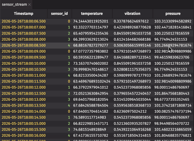
This creates a table that grows by one row every 500 milliseconds. Each row contains readings from one of five sensors, with about 10% of readings showing anomalous behavior.

Step 2: Train an anomaly detection model

Now let's train a model to recognize anomalies. We'll use scikit-learn's Isolation Forest — an unsupervised algorithm that learns what "normal" looks like and flags outliers.

First, generate some training data (normal readings only):

Result:

The model learns the distribution of normal sensor readings. In production, anything that deviates significantly from this distribution gets flagged as an anomaly.

Now the interesting part — connecting this trained model to live data without reprocessing the entire table every time a new row arrives.

Step 3: Deploy with deephaven.learn

Now we connect the trained model to the live stream. The learn function uses a gather-compute-scatter pattern that processes only changed rows:

1. Gather: Extract data from table columns into NumPy arrays.
2. Compute: Run your model on the gathered data.
3. Scatter: Write results back into new table columns.

Let's break down what's happening:

• Input specifies which columns to gather and how. Our gather_features function converts the three sensor columns into a NumPy array.
• model_func is called on each batch of gathered data. Our model returns 1 for normal readings, -1 for anomalies.
• Output specifies how to scatter results back to the table. The scatter_predictions function extracts each prediction by index.
• batch_size controls how many rows are processed together. Larger batches are more efficient; smaller batches give faster response times.

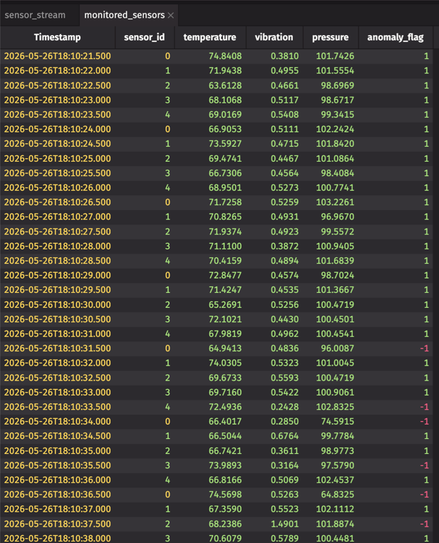
Step 4: Watch it work

The monitored_sensors table now updates in real-time. Every time new sensor readings arrive, deephaven.learn automatically:

1. Gathers the new rows (not the entire table — just the changes).
2. Runs the model on that batch.
3. Scatters the predictions into the anomaly_flag column.

Let's add a human-readable status and filter to see just the anomalies:

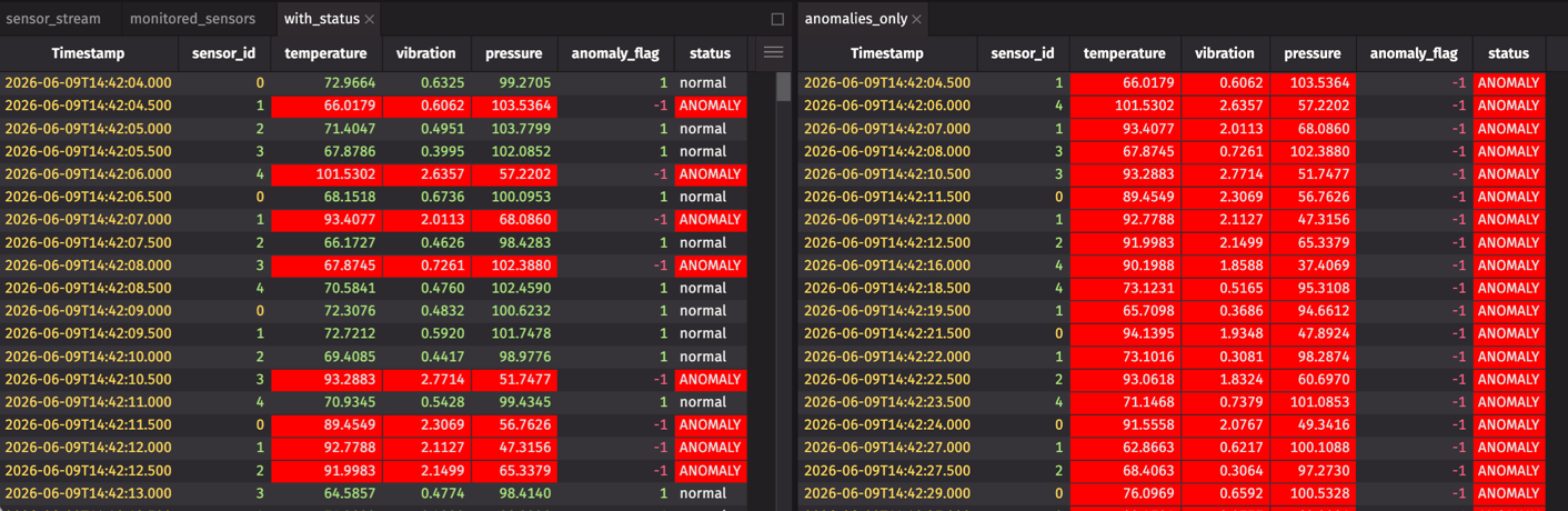
You now have three live tables:

• sensor_stream — raw sensor readings
• with_status — readings with anomaly predictions
• anomalies_only — only the flagged anomalies

As new data streams in, anomalies are flagged within milliseconds of arrival.

Why this matters

Traditional batch inference doesn't scale with streaming data. Every time new rows arrive, you'd have to reload the entire dataset and rerun predictions on everything. Latency grows with table size.

deephaven.learn only processes the rows that changed since the last update cycle. This makes it practical to deploy any trained model — scikit-learn, PyTorch, TensorFlow, XGBoost — on high-volume streams with millisecond-level latency.

The same pattern works beyond anomaly detection: fraud scoring, demand forecasting, image classification, quality control, and more. Train once, deploy on a stream, let it run.

Try it yourself

This tutorial requires a local installation — the browser demo doesn't include scikit-learn. Follow the pip quickstart to get started, then check the deephaven.learn docs for the full API.

What to try next: Replace Isolation Forest with your own model. The gather-compute-scatter pattern works with any Python function, including sklearn estimators, PyTorch modules, TensorFlow models, and XGBoost classifiers. Change model_func and you're done.

A few ideas:

• Connect to a live data feed instead of simulated sensors.
• Add a rolling window aggregation before the model.
• Chain multiple models (feature extraction → classification → alerting).

The scikit-learn integration guide covers more patterns. Questions? Join us on Slack.