Detect credit card fraud with Deephaven

Credit card fraud causes billions of dollars in damages each year. The most infamous cases have affected tens to hundreds of millions of consumers in single attacks through the unlawful exposure of personally identifiable information (PII) related to credit cards. Isolated cases are also common, and can be caused by a variety of methods including skimming, social engineering, and application fraud.

In order to protect their customers, credit card companies rely on fraud detection and prevention software to analyze credit card purchases. These programs look for unusual or unexpected patterns to classify them as possibly fraudulent. In this blog, we propose our own real-time credit card fraud detection solution using Python with Deephaven.

The code in this blog uses SciKit-Learn, which does not come with Deephaven's base images. To run this code, ensure you have the module installed. Here's how you can Install and use Python packages. We also have a guide for How to use SciKit-Learn in Deephaven.

The data set

We use the credit card fraud dataset that is publicly available on Kaggle and in Deephaven's Examples repository.

The data set consists of 284,807 credit card purchases over the course of 48 hours by European cardholders. Only 492 of these purchases are fraudulent, making this data set heavily imbalanced by the valid purchases. Due to the sensitive nature of the data, the purchase metrics, which consist of 28 variables (named V1 through V28), have been transformed and anonymized so that there is no identifiable information contained within them.

Let's assume the following basic points:

• Fraudulent purchases are spatial outliers among their valid counterparts.
• Not all purchase metrics will help us obtain a good solution.
• Incorrectly classifying a valid purchase as fraudulent is better than incorrectly classifying a fraudulent purchase as valid.

The first assumption is somewhat naive, but can produce adequate results with proper preparation and data exploration.

Data exploration

We first have to import the data into memory.

# Required imports
from deephaven import read_csv

# Read the CSV file into a Deephaven table
creditcard = read_csv("/data/examples/CreditCardFraud/csv/creditcard.csv")

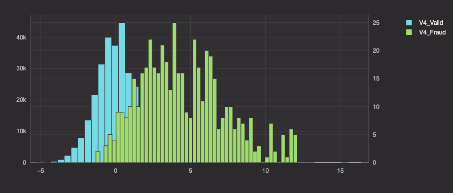
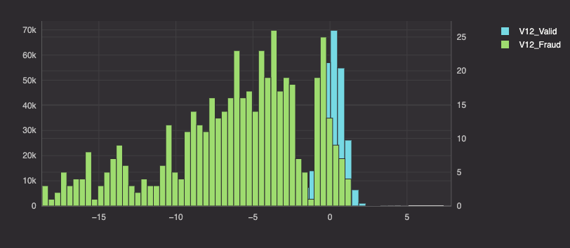
Before we try to rid the world of credit card fraud, let's explore the data. We've decided to approach the problem with the idea that fraudulent purchases can be considered spatial outliers in the data. We can use Deephaven's plotting capabilities to check our assumption. A histogram plot can show us how similar or different valid and fraudulent purchases are for any given purchase metric.

The code below defines a function that will create a histogram plot that shows how the distribution of points differs between valid and fraudulent purchases for any of the anonymized purchase metrics in the table.

# Required imports
from deephaven.plot import Figure

def plot_valid_vs_fraud(col_name):
    # Set the creditcard table as global to make sure we can access it for the plot
    global creditcard

    # Make sure the input corresponds to a column
    allowed_col_names = [item for item in range(1, 29)] + ["V" + str(item) for item in range(1, 29)]
    if col_name not in allowed_col_names:
        raise ValueError("The column name you specified is not valid.")
    if isinstance(col_name, int):
        col_name = "V" + str(col_name)

    # Some convenience variables for plotting
    num_valid_bins = 50
    num_fraud_bins = 50
    valid_label = col_name + "_Valid"
    fraud_label = col_name + "_Fraud"
    valid_string = "Class = 0"
    fraud_string = "Class = 1"

    # Create a fancy histogram plot
    fig = Figure()
    new_fig = fig.\
        plot_xy_hist(series_name=valid_label, t=creditcard.where([valid_string]), x=col_name, nbins=num_valid_bins).\
        x_twin().\
        plot_xy_hist(series_name=fraud_label, t=creditcard.where([fraud_string]), x=col_name, nbins=num_fraud_bins)
    valid_vs_fraud = new_fig.show()
    return valid_vs_fraud

There are 28 columns of data to explore, so we won't show all of them here. Histogram plots of columns V4, V12, and V14 show significant differences in how valid and fraudulent purchases are distributed along those spaces. Thus, we will use these three columns for our analysis.

valid_vs_fraud_V4 = plot_valid_vs_fraud("V4")
valid_vs_fraud_V12 = plot_valid_vs_fraud("V12")
valid_vs_fraud_V14 = plot_valid_vs_fraud("V14")

Moving forward, our queries will analyze only the following columns:

• Time
• V4
• V12
• V14
• Class

The solution

The clustering algorithm

Ok, so we want to classify spatial outliers. How can this be done with the data at hand?

We're going to use DBSCAN - Density Based Spectral Clustering of Applications with Noise. Why use DBSCAN?

• DBSCAN can find arbitrarily shaped clusters - we know little about what our cluster(s) will look like.
• DBSCAN can find an arbitrary number of clusters - we want one single cluster.
• DBSCAN is robust to outliers - which is exactly what we're looking for.
• SciKit-Learn offers an intuitive and highly customizable DBSCAN method.

SciKit-Learn's implementation, sklearn.cluster.DBSCAN, has two required inputs:

• A neighborhood distance.
• The number of neighbors to be considered part of a cluster.

There are a number of additional optional input parameters that can be specified, although we won't cover them here since we won't use them.

We're going to use four hours worth of purchase data to fit our DBSCAN model, and then four hours of live data on which we will make predictions. These two sets will be separated by 24 hours. Once we split the data, we need to set our model's input parameters.

Our training set will consist of purchases that occur between hours 12 and 16. Then, our testing set will consist of the four hour window that occurs 24 hours later - purchases that occur between hours 36 and 40. We are separating our training and testing sets by 24 hours because we expect purchases to have similarities on a per-day basis.

Choosing the neighborhood distance

The first input parameter we must choose is the neighborhood distance. In DBSCAN, the neighborhood distance corresponds to a radius around a given point. Thus, a "neighborhood" around a point is a sphere with the point at its center. Making an informed decision about the neighborhood distance will improve the accuracy of a DBSCAN model.

A DBSCAN neighborhood distance is typically chosen based upon every point's distance to its nearest neighbor. If these nearest neighbor distances are placed in ascending order, a curve is created. The most common choice of neighborhood distance is at the "knee" or "elbow" of the curve. Let's create this curve, plot it, and pick our neighborhood distance.

from deephaven.pandas import to_pandas, to_table

from sklearn.neighbors import KDTree as kdtree
import pandas as pd
import numpy as np

# Remove unwanted columns and split into train/test sets
creditcard = creditcard.select(formulas=["Time", "V4", "V12", "V14", "Amount", "Class"])
train_data = to_pandas(creditcard.where(filters=["Time >= 43200 && Time < 57600"]))
test_data = to_pandas(creditcard.where(filters=["Time >= 129600 && Time < 144000"]))

data = train_data[["V4", "V12", "V14"]].values

# Get nearest neighbor distances using a K-D tree
tree = kdtree(data)
dists, inds = tree.query(data, k=2)

# Sort the nearest neighbor distances in ascending order
neighbor_dists = np.sort(dists[:, 1])

x = np.array(range(len(neighbor_dists)))

# Turn our x and y (sorted neighbor distances) into a Deephaven table
nn_dists = pd.DataFrame({"X": x, "Y": neighbor_dists})
nn_dists = to_table(nn_dists)

# Plot the last few hundred points so we can see the "elbow"
fig = Figure()
dist_fig = fig.plot_xy(series_name="Nearest Neighbor Distance", t=nn_dists.where(filters=["X > 30000"]), x="X", y="Y")
neighbor_dists = dist_fig.show()

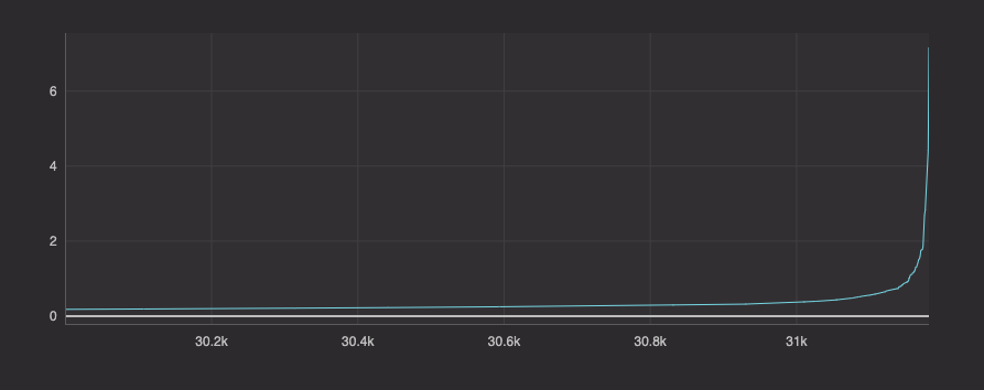
There are 31,181 purchases in our training window. The elbow of the curve occurs right near the end of our plot, so we cut out the first 30,000 points from our plot. The elbow of this curve occurs where the neighborhood distance is almost exactly one. Thus, we'll use 1 as our first input to DBSCAN.

The number of neighbors

The second input parameter we must choose is the number of neighbors. This input corresponds to the number of other points that live within the neighborhood distance of a given point for it to be considered part of a cluster. Thus, DBSCAN checks every point in the set to see how many other points reside within its neighborhood. If a point has greater than or equal to the specified number of neighbors, it's part of a cluster. If less, the point is considered noise. There is some special handling done to discern clusters from one another, but that doesn't apply to this problem. What we want is one single cluster of valid purchases. Any point not belonging to that single cluster is then considered a fraudulent purchase.

There is more flexibility when choosing this parameter. The general rule of thumb is that this value should be higher than the number of dimensions in the data. We have 3 dimensions. We'll use 10 for the number of neighbors based on some trial and error.

To see the effect of each input on the training data, consider modifying them by running the fitting the model code down below, and seeing how they affect the model's accuracy.

Fitting the model and using the fitted model

We'll fit the model on four hours of data, then use the fitted model to predict fraud on a four hour window that occurs 24 hours later. We do this because we expect a degree of similarity between the number of purchases and the rate of fraud during the same time periods on different days.

If DBSCAN were to be used in a real fraud system, it could be wise to train models for various phases of the day, and then deploy these various models at the time of day for which they are most effective.

The code

Ok, lots of talk but little code so far. Let's get into the actual solution as it works in Deephaven.

Fitting the model

We first need to fit the model to our data. Our training features consist of columns V4, V12, and V14. Our training targets are in the Class column. For training, we want hours 12, 13, 14, and 15.

Let's fit the model using this training data and the inputs we specified earlier.

There's quite a bit going on in the code below. Let's break it down into steps:

• Import everything we need for static and real-time analysis.
• Read the CSV data into memory and create training and testing tables from it.
• Add timestamps to the testing table for later use.
• Create a function to fit a DBSCAN model with our chosen inputs to the training set.
• Construct functions to scatter and gather data to and from Deephaven tables.
• Apply DBSCAN to the training data via the learn function.
• Check how the model performs.

# Deephaven imports
from deephaven.time import plus_period, to_datetime, to_period
from deephaven.learn import gather
from deephaven import learn

# Python imports
from sklearn.neighbors import KDTree as kdtree
from sklearn.cluster import DBSCAN as dbscan
import pandas as pd
import numpy as np
import scipy as sp

# Split the credit card table into train/test sets
train_data = creditcard.where(filters=["Time >= 43200 && Time < 57600"])
test_data = creditcard.where(filters=["Time >= 129600 && Time < 144000"])

# This base time will be used to generate time stamps
base_time = to_datetime("2021-11-16T00:00:00 NY")

# This function will create a timestamp column from the time offset column
def timestamp_from_offset(t):
    global base_time
    db_period = "T{}S".format(int(t))
    return plus_period(base_time, to_period(db_period))

# Add a timestamp column to the test data for later replay
test_data = test_data.update(formulas=["TimeStamp = (DateTime)timestamp_from_offset(Time)"])

# This placeholder will be replaced by our trained DBSCAN model
db = 0

# A function to apply DBSCAN with eps = 1 and min_samples = 10
def perform_dbscan(data):
    global db
    db = dbscan(eps=1, min_samples=10).fit(data)
    return db.labels_

# Our gather function for DBSCAN
def dbscan_gather(rows, cols):
    return gather.table_to_numpy_2d(rows, cols, np_type=np.double)

# Our scatter function for DBSCAN
def dbscan_scatter(data, idx):
    if data[idx] == -1:
        data[idx] = 1
    return data[idx]

# Perform DBSCAN on our train_data table
clustered = learn.learn(
    table = train_data,
    model_func = perform_dbscan,
    inputs = [learn.Input(["V4", "V12", "V14"], dbscan_gather)],
    outputs = [learn.Output("PredictedClass", dbscan_scatter, "short")],
    batch_size = train_data.size
)

# Split DBSCAN guesses (correct and incorrect) into separate tables
dbscan_correct_valid = clustered.where(filters=["Class == 0 && PredictedClass == 0"])
dbscan_correct_fraud = clustered.where(filters=["Class == 1 && PredictedClass == 1"])
dbscan_false_positives = clustered.where(filters=["Class == 0 && PredictedClass == 1"])
dbscan_false_negatives = clustered.where(filters=["Class == 1 && PredictedClass == 0"])

# Report the accuracy of the model
print("DBSCAN guesses valid - correct! " + str(dbscan_correct_valid.size))
print("DBSCAN guesses fraud - correct! " + str(dbscan_correct_fraud.size))
print("DBSCAN guesses valid - wrong! " + str(dbscan_false_positives.size))
print("DBSCAN guesses fraud - wrong! " + str(dbscan_false_negatives.size))

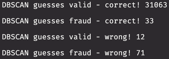
Sweet! Let's break down the model's performance:

• 31063 out of 31075 valid purchases are correctly identified (>99%).
• 33 out of 45 fraudulent purchases are correctly identified (73%).
• 12 fraudulent purchases are misidentified as being valid - these are false negatives (27%).
• 71 valid purchases are misidentified as being fraudulent - these are false positives (<1%).

These results are pretty good. Let's move forward!

Real-time fraud detection

We already have the test_data table in memory. We want to replay it in real time based off the timestamps we created in its DateTime column. We can do this using Replayer.

DBSCAN isn't a model built for real-time processing. We must leverage what we know about the DBSCAN model we've created on our training data in order to create a real-time method that utilizes our model:

• The fitted model has one cluster.
• A point is part of this single cluster if it has 10 neighbors within a radius of 1.
• A point is not part of the cluster if any of its nearest 10 neighbors are further than a distance of 1 away from it.

With this knowledge, we can compare test data coming in real time to our training data and see if it is part of the single cluster.

The code below can be broken into steps:

• Replay the test_data table in real time.
• Construct a function to predict the validity of incoming purchases using the training data and our model.
• Create function to scatter and gather data to and from a Deephaven table.
• Use learn to apply our model to the real-time updating table.
• Create derived tables that show how our models perform in real time.

from deephaven.replay import TableReplayer

start_time = to_datetime("2021-11-17T12:00:00 NY")
end_time = to_datetime("2021-11-17T16:01:00 NY")

# Replay the test_data table
test_data_replayer = TableReplayer(start_time, end_time)
creditcard_live = test_data_replayer.add_table(test_data, "TimeStamp")
test_data_replayer.start()
creditcard_live = creditcard_live.view(formulas = ["Time", "V4", "V12", "V14", "Amount", "Class"])

# A function to place new observations into our existing clusters
def dbscan_predict(X_new):
    n_rows = X_new.shape[0]
    data_with_new = np.vstack([data, X_new])
    tree = kdtree(data_with_new)
    dists, points = tree.query(data_with_new, 10)
    dists = dists[-n_rows:]
    detected_fraud = [0] * n_rows
    for idx in range(len(dists)):
        if any(dists[idx] > 1):
            detected_fraud[idx] = 1
    return np.array(detected_fraud)

# A function to gather data from a Deephaven table into a NumPy array
def table_to_numpy(rows, cols):
    return gather.table_to_numpy_2d(rows, cols, np_type=np.double)

# A function to scatter data back into an output table
def scatter(data, idx):
    return data[idx]

predicted_fraud_live = learn.learn(
    table = creditcard_live,
    model_func = dbscan_predict,
    inputs = [learn.Input(["V4", "V12", "V14"], table_to_numpy)],
    outputs = [learn.Output("PredictedClass", scatter, "short")],
    batch_size = 1000
)

dbscan_correct_valid = predicted_fraud_live.where(filters=["PredictedClass == 0 && Class == 0"])
dbscan_correct_fraud = predicted_fraud_live.where(filters=["PredictedClass == 1 && Class == 1"])
dbscan_false_positive = predicted_fraud_live.where(filters=["PredictedClass == 1 && Class == 0"])
dbscan_false_negative = predicted_fraud_live.where(filters=["PredictedClass == 0 && Class == 1"])

Conclusion

Now we have our fitted DBSCAN model classifying fraud in real time! We can see that as new rows are added, our model is accurately identifying fraud as it comes in! However, our model doesn't catch every fraudulent purchase. Perhaps a DBSCAN model with different parameters would work better? There may be different models that are better suited to this problem altogether.

Nevertheless, we are able to construct a relatively simple model and that works pretty well on a difficult problem. Extending the model to use Deephaven tables is intuitive and easy, and extending a static solution to work on real-time live data is equally so.

What kind of data science problems can you solve on live data using Deephaven? There's an innumerable wealth of data out there that needs processing, and Deephaven is an excellent tool for doing just that.