
Towards real-time epileptic seizures forecasts

· 11 min read
DALL·E prompt: A thunder cloud shaped like a human brain with lighting bolts coming out of it, by René Magritte
Stacy Serebryakova
Making predictions with an LSTM network with Deephaven

Machine learning techniques have an ever-increasing importance in healthcare. Some key applications include medical image classification, treatment recommendations, disease detection, and prediction. This blog discusses predicting seizures in epileptic patients through binary classification.

You don't need to be a neuroscience expert to develop a basic working prototype of a seizure prediction model. To classify electroencephalogram (EEG) signals we will use a long short-term memory (LSTM) recurrent neural network (RNN) with Deephaven.

Deephaven is ideally suited for this task - its images for AI/ML in Python make using TensorFlow easy (for more information, please see our guide). Besides, in real-world applications, EEG data is generated in the form of a stream, such as neural activity records from brain implants, sensors, or wearable devices. Deephaven's streaming tables are a natural choice to make real-time predictions.

Background

Seizures are like storms in the brain — sudden bursts of abnormal electrical activity that can cause disturbances in movements, behavior, feelings, and awareness. There is no regularity in their occurrence, so doctors have no way of telling people with epilepsy when the next seizure might happen - in 20 hours, in 20 days, or 20 weeks after a previous one. 25% of the patients with epilepsy are drug-resistant and have to live with the threat of a sudden seizure at any time.

For many years, neuroscientists thought seizures began abruptly, just a few seconds before clinical attacks. Recent research has shown that seizures are not random events and develop minutes to hours before clinical onset. There are 4 states of brain activity: interictal (between seizures), preictal (before seizure), ictal (seizure), and post-ictal (after seizures). Over the last few years, significant research has demonstrated the existence and accurate classification of the preictal brain state.

Dataset

The latest studies show that seizures can be forecast 24 hours in advance — and in some patients, up to three days prior. In this work, we will not be so ambitious. Instead, we will try to predict the risk of a seizure within 10-minute intervals. We will be using a dataset from the American Epilepsy Society Seizure Prediction Challenge on Kaggle. It is EEG data from the NeuroVista seizure advisory system implant.

Each epilepsy patient has their own specific pre-seizure signatures, so we will be using records of brain electrical activity only for one patient from the dataset for the sake of time. The goal of our experiment is to distinguish between 10-minute-long data clips covering an hour before a seizure (i.e., preictal clips), and 10-minute EEG clips with no oncoming seizures (interictal clips).

Load the data

Let's start by loading the EEG data:

import glob

CLIP_PATH = "/data/Patient_1/"

def get_clips(data_folder):

# Get all clips
clips = os.listdir(data_folder)

# Preictal recordings - time-series segments of the measurement before a seizure occura
clips_preictal = glob.glob(os.path.join(data_folder, "*preictal*"))

# Interictial segments - segments with no oncoming seizures
clips_interictial = glob.glob(os.path.join(data_folder, "*interictal*"))

return clips_interictial, clips_preictal


# Get EEG recordings
clips_interictal, clips_preictal = get_clips(data_folder = CLIP_PATH)

For our patient, EEG data was recorded with 15 channels (15 electrodes) and a sampling rate of 5000 Hz. In each channel, a sampling frequency (5000 Hz) determines how many data samples represent 1 second of EEG data. The sampling frequency multiplied by the total measurement time per clip (~600 seconds in our example) determines the length of each time series (around 3,000,000).

Features

There are various signal processing methods to engineer features from the raw EEG data. The Kaggle competition winners used the power spectral band, the signal correlation between EEG channels and eigenvalue of the correlation matrix, Shannon's entropy, and many more.

In this blog, we want to keep it simple - we won't dive deep into complex signal processing theories and neuroscience interpretations; instead, we will only perform a 1d convolution on the raw measurements.

For our LSTM network, we want to use TensorFlow, which requires input as a tensor with the shape (N, seq_len, n_channels) where:

  • N is the number of data points.
  • seq_len is the sequence length for time-series.
  • n_channels is the number of channels.

The problem we face here is that the raw data sequence is very long for the LSTM network. In our example, there are approximately 3,000,000 points in time. This is very long, and typical LSTM cells cannot be trained for such a long series. Therefore, we are going to use 1d convolutions with averages to reduce the number of points. This results in a shorter time series that we can use as an input to an LSTM network. Our approach is based on the code available on this GitHub repository:

Click to see the code!
import os
import numpy as np
from scipy.io import loadmat

# Construct LSTM sequences from one segment
def lstm_sequence(input_segment, target, sampling_freq, window, stride, block_s = 60):
""" Function for generating blocks of LSTM input tensors
input_segment : The EEG segment
target : 1/0 (preictal/interictial); None for test
sampling_freq : Samplig frequency
window : Window size for 1d convolutions on each block
stride : Stride size of the 1d convolution
block_s : Size of the block in seconds (default = 60)
"""

# Dimensions
n_channels, T_segment = input_segment.shape

# Determine block dimensions
block_len = sampling_freq * block_s # Length of each block
n_blocks = (T_segment-1) // block_len # Number of blocks
blocks = [block for block in range(0,(n_blocks+1)*block_len,block_len)]

# Determine the sequence length for LSTM
div = (block_len - window)%stride
if (div != 0):
pad = stride - div # Size of padding neded
else:
pad = 0

seq_len = (block_len + pad - window) // stride

# Initiate tensor
X = np.zeros((n_blocks, seq_len, n_channels))

# Loop over blocks and fill X
for ib in range(n_blocks):
# Get block
data_block = input_segment[:, blocks[ib]:blocks[ib+1]]

# Pad if necessary
if (pad !=0):
data_block = np.concatenate((data_block, np.zeros((n_channels, pad))), axis=1)

# 1d convolution by mean
index = 0
for j in range(seq_len):
X[ib, j, :] = np.mean(data_block[:, (index+j):(index+j+seq_len)], axis = 1)

# Fill in the target
if (target == 1):
Y = np.ones(n_blocks)
elif(target == 0):
Y = np.zeros(n_blocks)
else:
Y = None

return X, Y, n_blocks

# Collect all the segments to build a tesnsor input for LSTM
def lstm_build_input(clips, target, window, stride, block_s = 60):
""" Collect all the data and build sequences for LSTM
clips : List of clips
target : 1/0 (preictal/interictial); None for test set
window : Window size for 1d convolutions
stride : Length of the stride in 1d convolution
block_s : Size of the block in seconds (default = 60)
"""

# Number of clips
n_clips = len(clips)

# Loop over all clips and store data
iclip = 0
for file in clips:
clip = loadmat(file)
segment_name = list(clip.keys())[3] # Get segment name
input_segment = clip[segment_name][0][0][0] # Get electrode data
sampling_freq = np.squeeze(clip[segment_name][0][0][2]) # Sampling frequency

# Get number of channels
n_channels = clip[segment_name][0][0][0].shape[0]

# Get tensor input and targets from blocks
X, Y, n_blocks = lstm_sequence(input_segment, target, sampling_freq, window, stride, block_s)

# Concatenate the tensor and target vector
if (iclip == 0):
X_train = X
Y_train = Y[:,None] if Y is not None else None
else:
X_train = np.vstack((X_train,X))
Y_train = np.vstack((Y_train,Y[:,None])) if Y is not None else None

iclip +=1

return X_train, Y_train


# Window, stride and block_s
window = 16000
stride = 100
block_s = 60

X_1, Y_1 = lstm_build_input(clips_preictal, 1, window, stride)
X_0, Y_0 = lstm_build_input(clips_interictal, 0, window, stride)

# Scale the data
X_1 = X_1 / np.max(np.abs(X_1), axis=1)[:,None,:]
X_0 = X_0 / np.max(np.abs(X_0), axis=1)[:,None,:]

# Combine the data
X = np.concatenate((X_0, X_1), axis = 0)
Y = np.concatenate((Y_0, Y_1), axis = 0)
Y = np.squeeze(Y)

print("Data shape = ", X.shape)

After averaging, our data shape is (612, 2840, 15), which is an acceptable value a typical LSTM network can handle.

It is always a good idea to normalize the data:

# Normalize
X = X / np.max(np.abs(X), axis=1)[:,None,:]

# Shuffle
np.random.seed(1)
shuffle = np.random.choice(np.arange(len(Y)), size=len(Y), replace=False)
X = X[shuffle]
Y = Y[shuffle]

Build the model

Finally, we are ready to build our RNN model for predictions:
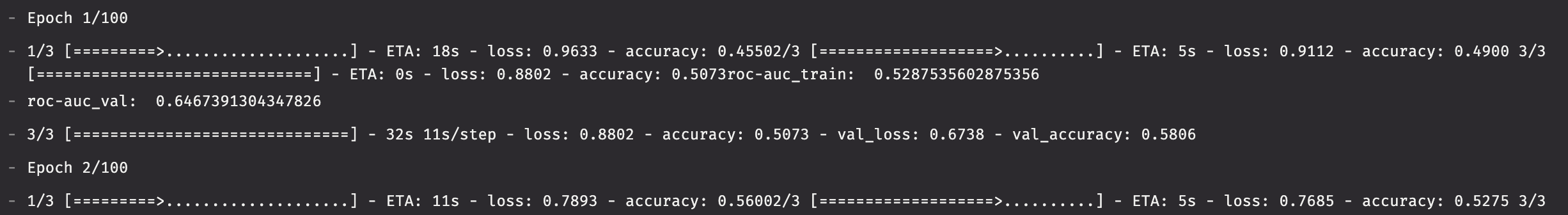
import tensorflow as tf
from tensorflow import keras
from tensorflow.keras import layers

model = keras.Sequential()
model.add(layers.Input(shape=(2840, 15)))
model.add(layers.LSTM(64))
model.add(layers.BatchNormalization())
model.add(layers.Dense(1, activation='sigmoid'))

Train the model

Now let's train our model with Deephaven tables. This requires a few additional functions:

Click to see the code!
from deephaven import learn
from deephaven.learn import gather
from deephaven import numpy
from keras.callbacks import Callback

from sklearn.model_selection import train_test_split
from sklearn.metrics import roc_auc_score


class RocCallback(Callback):
def __init__(self,training_data,validation_data):
self.x = training_data[0]
self.y = training_data[1]
self.x_val = validation_data[0]
self.y_val = validation_data[1]

def on_train_begin(self, logs={}):
return

def on_train_end(self, logs={}):
return

def on_epoch_begin(self, epoch, logs={}):
return

def on_epoch_end(self, epoch, logs={}):
y_pred_train = model.predict(self.x)
roc_train = roc_auc_score(self.y, y_pred_train)
y_pred_val = model.predict(self.x_val)
roc_val = roc_auc_score(self.y_val, y_pred_val)
print('roc-auc_train: ', roc_train)
print('roc-auc_val: ', roc_val)
return

def on_batch_begin(self, batch, logs={}):
return

def on_batch_end(self, batch, logs={}):
return


# Function that trains the model
def train_model(X, Y):
X = X.reshape(X.shape[0], -1, n_channels) # reshape DH table to 3d numpy array
X_train, X_valid, Y_train, Y_valid = train_test_split(X, Y, stratify=Y, test_size = 0.1)
roc = RocCallback(training_data=(X_train, Y_train), validation_data=(X_valid, Y_valid))
model.compile(loss='binary_crossentropy', optimizer="adam", metrics=["accuracy"])
model.fit(X_train, Y_train, validation_data=(X_valid, Y_valid), callbacks=[roc], batch_size = 200, epochs=100)

# Function that gets the model's predictions on input data
def predict_with_model(X):
X = X.reshape(X.shape[0], -1, n_channels) # reshape DH table to 3d numpy array
Y_pred = model.predict(X, batch_size=200)
return Y_pred

# Function to gather data from table columns into a NumPy array of doubles
def table_to_array_double(rows, cols):
return gather.table_to_numpy_2d(rows, cols, np_type=np.double)

# Function to gather data from table columns into a NumPy array of integers
def table_to_array_int(rows, cols):
return gather.table_to_numpy_2d(rows, cols, np_type=np.intc)

# Function to extract a list element at a given index
def get_predicted_class(data, idx):
return data[idx]

# Split the data into training and test datasets
X_train, X_test, Y_train, Y_test = train_test_split(X, Y, stratify=Y, test_size = 0.2)

# Convert numpy arrays X_train and Y_train to DH table X_table
n_rows = X_train.shape[0]
n_cols = X_train.shape[1] * X_train.shape[2]
column_names = ['Col_'+str(i) for i in range(n_cols)]
X_reshaped = X_train.reshape(n_rows, n_cols)
X_table = numpy.to_table(X_reshaped, cols=column_names)

def add_class_col(index):
y_class = [int(i) for i in Y_train.tolist()]
return y_class[index]

X_table = X_table.update(["Class = (int)add_class_col(i)"])


# Train the model
learn.learn(
table=X_table,
model_func=train_model,
inputs=[learn.Input(column_names, table_to_array_double), learn.Input(["Class"], table_to_array_int)],
outputs=None,
batch_size=200
)


# Convert numpy array X_test to DH table X_table_test
X_reshaped_test = X_test.reshape(X_test.shape[0], n_cols)
X_table_test = numpy.to_table(X_reshaped_test, cols=column_names)

# Use the learn function to create a new table that contains predicted values
predicted = learn.learn(
table=X_table_test,
model_func=predict_with_model,
inputs=[learn.Input(column_names, table_to_array_double)],
outputs=[learn.Output("PredictedClass", get_predicted_class, "int")],
batch_size=200
)

To evaluate our model, we calculated the area under the ROC curve (AUC) - the same metric that was used to judge submissions in the Kaggle Seizure Prediction Challenge. For our validation dataset, we got AUC = 0.8. Of course, it should ideally be closer to 1 for a good classifier. But our model is just a toy example we built with limited domain knowledge in neuroscience and without using complex signal processing procedures and feature engineering.

img

Real-time predictions

As mentioned before, one of Deephaven's biggest advantages is the ability to deal with numerous real-time data feeds. To simulate the real-time feed, we can use a TableReplayer:

from deephaven.replay import TableReplayer
from deephaven import time as dtu
from deephaven.time import to_datetime
from deephaven import numpy

# use our test data to simulate real-time feed
X_live = X_test
n_rows = X_live.shape[0]
n_cols = X_live.shape[1] * X_live.shape[2]
X_live = X_live.reshape(n_rows, n_cols)

# convert numpy array to DH table
X_live = numpy.to_table(X_live, cols=column_names)

start_time = dtu.to_datetime("2022-01-01T00:00:00 NY")
def add_datetime_col(index):
return dtu.plus_period(start_time, dtu.to_period(f"T{index}S"))

X_live = X_live.update(["Timestamp = (DateTime)add_datetime_col(i)"])

# replay historical data
start_time = to_datetime("2022-01-01T00:00:00 NY")
end_time = to_datetime("2022-01-01T00:02:30 NY")

replayer = TableReplayer(start_time, end_time)
replayed_table = replayer.add_table(X_live, "Timestamp")
replayer.start()

predicted = learn.learn(
table=replayed_table,
model_func=predict_with_model,
inputs=[learn.Input(column_names, table_to_array_double)],
outputs=[learn.Output("PredictedClass", get_predicted_class, "int")],
batch_size=200
)

Though we trained our model on the static dataset, Deephaven can use the streaming data source to perform real-time classification:

Learn more