Built-in plotting API
Deephaven's built-in plotting API offers methods for creating real-time figures, plots, and charts from static and ticking tables. This guide provides an overview of its capabilities.
Note
The built-in plotting API is no longer under active development, and there are no plans for new patches, features, or fixes. Deephaven Express, the recommended choice for most plotting tasks, is available only in Python. From Groovy, the built-in plotting API is the way to plot Deephaven tables in code.
This guide covers the following plot types:
It also shows how to combine plots in subplots and make plots that users filter from the UI.
Each plotting method returns a Figure. You can call a plotting method such as plot on its own, as most examples on this page do, or on a figure created with figure. Either way, you chain more methods onto the result and finish with show.
XY series
XY series plots generally show values over a continuum, such as time. They can take the form of a line, a bar, an area, or a collection of points. The X axis shows the domain, while the Y axis shows the related values at specific points in the range.
You can create XY series plots using data from Deephaven tables with the following syntax:
plotis the method used to create an XY series plot.seriesNameis the name (as a string) you want to use to identify the series on the plot itself.sourceis the table that holds the data you want to plot.xColis the name of the column (as a string) that holds the X values.yColis the name of the column (as a string) that holds the Y values.showreturns a displayable version of the figure. Assign the result to a variable to see the plot in the console.
The example below creates an XY series plot of distance traveled over time during a metric-century bike ride. The where filter drops the rows where the rider was stopped.
Shared axes
You can compare multiple series over the same period of time by creating an XY series plot with shared axes. In the following example, two series create two line graphs on the same plot.
To add more series to the plot, chain more plot calls onto the figure.
Tip
To hide a series, click its name at the right of the plot. Click the name again to restore it.
Plot multiple series in a loop
It's common in data analysis to have multiple series that share an X axis. In that case, a for loop can add each series to the figure. The following example plots three different series on the same plot in a for loop.
Plot by a grouping column
The plotBy method plots a separate series for each value in a grouping column:
Category and OHLC plots have equivalent methods, described in Category: Plot by a grouping column and OHLC: Plot by a grouping column.
Multiple X or Y axes
When series in one plot have very different value ranges, a shared Y axis has to cover all of them, so the smaller series flatten and their changes become hard to see.
To fix this, add a second Y axis with the twinX method. twinX enables you to use one Y axis for some of the series being plotted and a second Y axis for the others, while sharing the same X axis:
- Series plotted before
twinXshare the left Y axis. - Series plotted after
twinXshare the right Y axis. - All series share the same X axis.
In the following example, distance reaches about 100,000 meters while speed stays below 70 KPH, so each series gets its own Y axis:
The left Y axis shows the value range for distance, and the right Y axis shows the value range for speed.
The twinY method enables you to use one X axis for one set of the values being plotted and a second X axis for another, while sharing the same Y axis:
Plot colors
Use lineColor to set a series' line color and pointColor to set its point color. Both accept a named color, such as "RED", or a color you build from red, green, blue, and alpha values with colorRGB. This example takes the Distance and Speed plot from Multiple X or Y axes and draws its lines in red and yellow:
For the full list of available colors, see Named colors.
Plot styles
The XY series plot in Deephaven defaults to a line plot. Use the plotStyle method to format XY series plots as area charts, stacked area charts, bar charts, stacked bar charts, scatter charts, or step charts.
In any of the examples below, you can pass another style name to plotStyle, such as "area", "stacked_area", or "step". Style names are not case-sensitive.
XY series as a stacked area plot
The following example stacks cadence on top of heart rate:
XY series as a scatter plot
The example below draws two series as points and styles each one:
plotStyle("scatter")draws each series as points.pointSize,pointColor, andpointShapeset the size, color, and shape of each series' points.twinXgives each series its own Y axis.chartTitlesets the chart's title.
XY series with markers on selected points
In the example below, a line plot of speed gets a marker at every point where the rider went faster than 40 KPH.
- The
twinmethod adds a second set of axes that shares both the X and Y axes. plotStyle("scatter")then gives those axes the scatter style, so the series plotted on them appears as markers over the line.
XY series as a step plot
In the example below, plotStyle("step") draws a step plot. The lineStyle method applies a LineStyle object to the series. The inner call, lineStyle(3), is a different method that builds a LineStyle with a width of 3.
Category
Use the catPlot method to create category plots, which display data values from different discrete categories.
To plot data from a Deephaven table, use the following syntax:
catPlotis the method used to create a category plot.seriesNameis the name (as a string) you want to use to identify the series on the plot itself.sourceis the table that holds the data you want to plot.categoryColis the name of the column (as a string) that holds the categories.valueColis the name of the column (as a string) that holds the values.showreturns a displayable version of the figure. Assign the result to a variable to see the plot in the console.
chartTitle sets the chart's title.
Shared axes
You can compare multiple series across the same categories by creating a category plot with shared axes. The following example reuses source from the Category example, adds a second table, sourceTwo, with the same Categories column, and plots both as bar graphs on one chart:
To add more series to the chart, chain more catPlot calls onto the figure.
Plot by a grouping column
The catPlotBy method plots a separate category series for each value in a grouping column:
Plot styles
By default, category plots draw values as vertical bars. Use the plotStyle method to draw them as stacked bars, a line, an area, or a stacked area instead.
In the example below, you can pass another style name to plotStyle, such as "area" or "stacked_area".
Category plot with stacked bars
The following example draws the two series from the category shared axes example as stacked bars:
Category histogram
Use the catHistPlot method to create category histograms, which show how often each discrete value (category) occurs.
To plot data from a Deephaven table, use the following syntax:
catHistPlotis the method used to create a category histogram.seriesNameis the name (as a string) you want to use to identify the series on the chart itself.sourceis the table that holds the data you want to plot.valueColis the name of the column (as a string) containing the discrete values.showreturns a displayable version of the figure. Assign the result to a variable to see the plot in the console.
To plot data from an array, use the following syntax:
valuesis the array containing the discrete values.
Histogram
Use the histPlot method to create histograms.
A histogram shows how frequently different data values occur. It divides the data into intervals (bins), counts the values in each bin, and draws each count as a vertical bar. Unlike bar charts (category plots), bars in histograms do not have spaces between them unless there is a gap in the data.
To plot data from a Deephaven table, use the following syntax:
histPlotis the method used to create a histogram.seriesNameis the name (as a string) you want to use to identify the series on the chart itself.sourceis the table that holds the data you want to plot.valueColis the name of the column (as a string) that holds the X values.nbinsis the number of intervals to use in the chart.showreturns a displayable version of the figure. Assign the result to a variable to see the plot in the console.
The histPlot method assumes you want to plot the entire range of values in the dataset. You can also set the minimum and maximum values of the range with rangeMin and rangeMax, respectively:
rangeMinis the smallest value (as a double) to include.rangeMaxis the largest value (as a double) to include.
To plot data from an array, use the following syntax:
xis the array that holds the X values.
As with a table, you can set the minimum and maximum values of the range with rangeMin and rangeMax:
OHLC
Use the ohlcPlot method to create Open, High, Low, and Close (OHLC) plots. These typically show four prices of a security or commodity per time slice: the open and close of the time slice, and the highest and lowest values reached during the time slice.
This plotting method requires a dataset that includes one column containing the values for the X axis (time), and one column for each of the corresponding four values (open, high, low, close).
To plot data from a Deephaven table, use the following syntax:
ohlcPlotis the method used to create an OHLC chart.seriesNameis the name (as a string) you want to use to identify the series on the chart itself.sourceis the table that holds the data you want to plot.timeColis the name of the column (as a string) that holds the X-axis values.openColis the name of the column (as a string) holding the opening price.highColis the name of the column (as a string) holding the highest price.lowColis the name of the column (as a string) holding the lowest price.closeColis the name of the column (as a string) holding the closing price.showreturns a displayable version of the figure. Assign the result to a variable to see the plot in the console.
The following example bins BTC trades into one-minute intervals and uses an aggregation to compute each interval's open, high, low, and close prices. The trades in the file are not in time order, so the example sorts them by Timestamp first. That way, AggFirst and AggLast return each interval's earliest and latest trade.
Plot by a grouping column
The ohlcPlotBy method plots a separate OHLC series for each value in a grouping column:
The following example bins BTC and ETH trades together, computes OHLC values for each instrument and interval, and plots one series per instrument:
All the series share one Y axis. ETH trades at about one-fourteenth of BTC's price, so its series looks flat next to BTC's. To give each series its own Y axis, plot them separately, as the next section shows.
Multiple series with separate Y axes
Like XY series plots, OHLC plots can show multiple series on one chart. The following example repeats the BTC binning from the OHLC example, adds a second series for ETH, and uses twinX to give ETH its own Y axis:
The second ohlcPlot call adds an ETH series built the same way as the BTC series. The twinX call between them gives ETH its own Y axis, so the left Y axis shows the BTC price scale and the right Y axis shows the ETH price scale.
Pie
Use the piePlot method to create pie charts, which show each category's share of the total as a slice of a circle.
To create a pie chart from a table, use the following syntax:
piePlotis the method used to create a pie chart.seriesNameis the name (as a string) you want to use to identify the series on the plot itself.sourceis the table that holds the data you want to plot.categoryColis the name of the column (as a string) that holds the categories.valueColis the name of the column (as a string) that holds the values.showreturns a displayable version of the figure. Assign the result to a variable to see the plot in the console.
Treemaps
Use the treemapPlot method to create treemap charts, which show hierarchical data as nested rectangles, where each item's area is proportional to its value.
From a formatted table
Your table may already have the structure treemapPlot requires. It needs at least two columns:
- An ID column, which identifies each item.
- A parent column, which names the item each one sits under.
Following the parents up from any item must end at one top-level value, called the root. The root doesn't need a row of its own. In the examples below, root appears only in the parent column. When your table has this structure, use the following syntax:
seriesNameis the name (as a string) you want to use to identify the series on the plot itself.sourceis the table that holds the data you want to plot.idsis the name of the column that holds the item IDs to use in structuring the treemap chart.parentsis the name of the column that holds each item's parent ID.valuesis the name of the column that sets how large each item is compared to the others.labelsis the name of the column that holds the display text to use instead of the raw ID.hoverTextsis the name of the column that holds the text to display when hovering over an item.colorsis the name of the column that holds the color to use for each item.showreturns a displayable version of the figure. Assign the result to a variable to see the plot in the console.
Only ids and parents are required. Pass null for any of the other columns you don't have. By default, each item takes its color from the theme, and its label is its ID.
The following example plots a table that already has this structure:
You can interact with this plot. Click a group header to expand that group, and click it again to return to the full view. Click an individual cell to expand its contents.
The same table also has value, hover text, and color columns. The following example uses them to display more information:
The table's Text column holds each stock's percent change rather than a name, so the example passes the ID column, Label, as labels too. With a column of display names, pass that column instead.
From a raw data table
Raw data often lacks the ID and parent columns that treemapPlot needs. The following example builds them with view, selectDistinct, and merge:
financialsis a view of the rawsourcetable with only theSymbol,Name,Sector, andMarketCapcolumns.sectorsis a table of the top-level distinct sectors in the raw data.sectorItemsis a table of the top-level sectors with label and color information associated with them.stockItemsis a table with all the stock items and their associated labels. ItsColorformula picks a color based on each stock's percent change.itemsmergessectorItemsandstockItemsinto the single table thattreemapPlotplots.sAndPTreemapis a treemap plot created with thetreemapPlotmethod.
Subplots
A figure can contain subplots: separate charts arranged in a grid by row and column number.
- A single plot with several series draws them all in one plot area, sharing at least one axis.
- Subplots give each chart its own section of the figure.
Use subplots when the datasets have different units or scales and you don't need to read them against each other. To overlay two series with different scales on one plot instead, see Multiple X or Y axes.
Define subplots
Set the number of subplots when you create a figure with figure. The arguments are the number of rows and the number of columns.
For a figure with only one plot, specifying the number of rows and columns is optional. A figure created with figure and no arguments grows to fit each chart added by a newChart call with no arguments.
Add subplots to a figure
After defining the figure's grid, add each subplot with a newChart call. Each newChart call creates a chart at a given row and column in the figure, and the plotting methods that follow it draw on that chart. Row and column indices start at 0.
For example, to stack two subplots vertically, give the figure two rows and one column.
One row, two columns
Let's instead place the subplots side by side by giving the figure one row and two columns. The series Y appears on the left, and Z on the right.
Different plot types
A single figure can handle multiple plot types as well as both static and real-time data.
Dynamic plots
A dynamic plot redraws to show only the rows that match the value a user picks in a paired filter control: Deephaven's Input Filter, Linker, or Dropdown Filter. To make a plot dynamic, use a SelectableDataSetOneClick as its data source.
oneClick
The oneClick method creates a SelectableDataSetOneClick from a table or a partitioned table:
pTableis a partitioned table containing the data. It must have at least one key column.tis the table containing the data.byColumnsis one or more column names (as strings) to make available for input filtering. At least one column is required.requireAllFiltersToDisplaycontrols whether the plot waits for filters. Whentrue, the plot displays data only after the user sets a filter on everybyColumnscolumn. Whenfalse, data displays before the user sets every filter. Overloads that omit this argument usetrue.
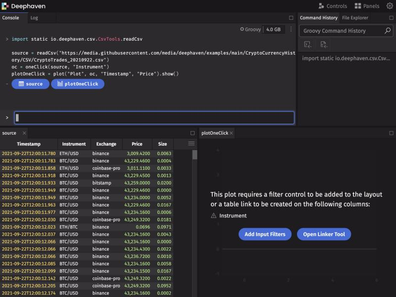
The following example uses oneClick(t, byColumns...), so the plot shows no data until you pick an Instrument value. Until then, the plot displays a message with Add Input Filters and Open Linker Tool buttons:
Input filters
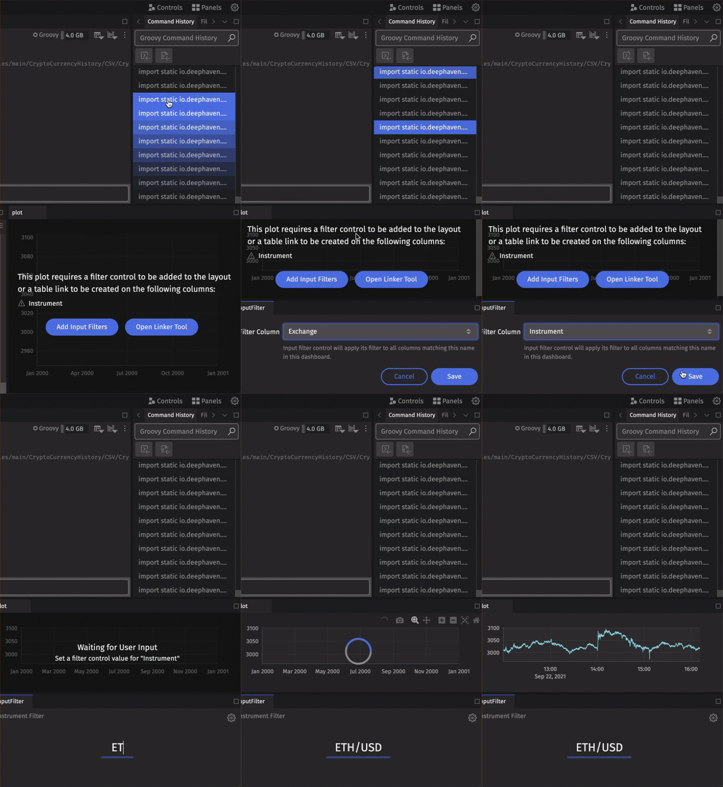
To pair your dynamic plot with an Input Filter, choose Input Filter from the Controls menu in the upper right-hand corner of the UI. If the plot is waiting for a filter, you can also click Add Input Filters on the plot itself.
Note
The Input Filter feature filters every open table in the dashboard that has a column with the same name and type as the filter column. It also filters every dynamic plot whose SelectableDataSetOneClick filters on such a column. That column is either a column listed in byColumns or a key column of the partitioned table passed to oneClick.
Linker tool
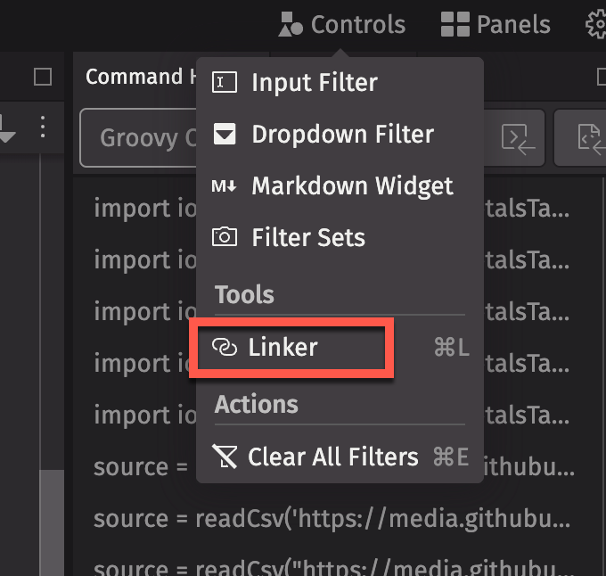
As an alternative to an Input Filter, you can use the Linker tool to pair a dynamic plot with a table. Choose Linker from the Controls menu. If the plot is waiting for a filter, you can also click Open Linker Tool on the plot.
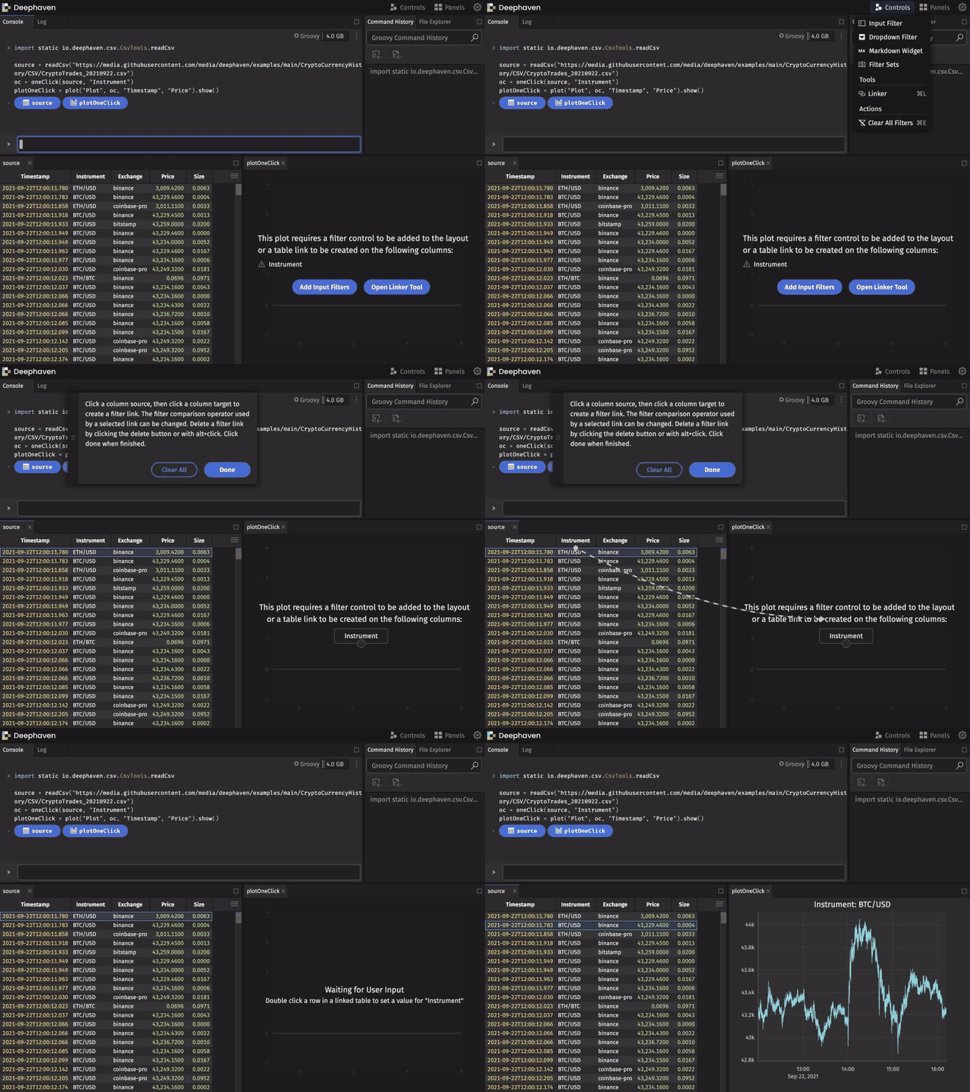
In the Linker, the table you filter from is the source table, and the dynamic plot is the target. Click the matching column in the source table, then click the column button on the dynamic plot. After that, double-clicking a row in the source table filters the plot to that row's value in the linked column.
Dropdown filters
You can also pair a dynamic plot with a Dropdown Filter, which filters on a value you choose from a list:
- Choose Dropdown Filter from the Controls menu.
- Under Source Column, select a column to supply the list of values.
- Under Filter Column, choose the column the plot's
SelectableDataSetOneClickfilters on. - Click Save, then pick a value from the list.
Related documentation
- How to use the Chart Builder
- Filter without writing queries
- Create and use partitioned tables
- Arrays
- Named colors
AggFirstAggLastAggMaxAggMinaggBycatHistPlotcatPlotcatPlotByemptyTablehistPlotintColmergenewTableohlcPlotoneClickpiePlotplotplotByplotStylereadCsvselectDistinctSelectableDataSetOneClicksortstringColsumBytimeTableupdateupdateViewviewwhereAxesJavadocchartTitleJavadoccolorRGBJavadocFigureJavadoclineColorJavadoclineStyleJavadocLineStyleJavadocnewChartJavadocohlcPlotByJavadocPlottingConvenienceJavadocpointColorJavadocpointShapeJavadocpointSizeJavadocshowJavadoctreemapPlotJavadoctwinJavadoctwinXJavadoctwinYJavadoc