Use SciPy

This guide will show you how to use SciPy in your Python queries in Deephaven.

Refer to our guide How to install Python packages for instructions on installing this package in Deephaven.

SciPy is an open-source scientific computing library for Python. It contains a large assortment of sub-packages with methods that can perform tasks in the following areas:

• Optimization
• Linear algebra
• Calculus
• Interpolation
• Transforms
• Signal processing
• Differential equations
• Multi-dimensional array processing

The above list is not comprehensive; SciPy's many sub-packages cover an even broader range of topics (see the Appendix at the bottom of this guide for a brief description of each). SciPy was built to operate on NumPy arrays, which we'll be using extensively in this guide. Check out How to use NumPy to learn more about how they work.

Examples

The examples below demonstrate using SciPy in a traditional Python setting, then extend them to use Deephaven. SciPy is a natural pair for deephaven.learn, so some of the corresponding Python queries with Deephaven use it. For more information on the learn submodule, check out How to use deephaven.learn.

Describe data

In this example, we'll use scipy.stats.describe to give basic insight into some data. The data we'll be describing is an ndarray with integer values from 0 to 99.

from scipy.stats import describe
import numpy as np

source = np.arange(100)
result = describe(source)
print(result)

To get these insights on data in a Deephaven table, we'll convert it to a NumPy array by using pandas.to_pandas and values. We can then use the method just as before.

from deephaven import empty_table, pandas
from scipy.stats import describe
import pandas as pd
import numpy as np

source = empty_table(100).update(formulas=["X = i"])
result = describe(np.squeeze(pandas.to_pandas(source).values))
print(result)

Compute the Airy function

In this example, we'll use scipy.special.airy to compute the Airy function of some values. In this case, we'll calculate the Airy function on values ranging from -20 to 0 in increments of 0.2.

from scipy.special import airy
import numpy as np

x = np.linspace(-20, 0, 101)
ai, aip, bi, bip = airy(x)

Let's extend this code to use Deephaven tables!

from deephaven import empty_table
from scipy.special import airy
import numpy as np

source = empty_table(101).update(formulas=["x = -20 + 20 * i / 100"])


def compute_airy(x):
    ai, aip, bi, bip = airy(x)
    return ai, aip, bi, bip


result = source.update(formulas=["y = compute_airy(x)"])

Filter a noisy signal

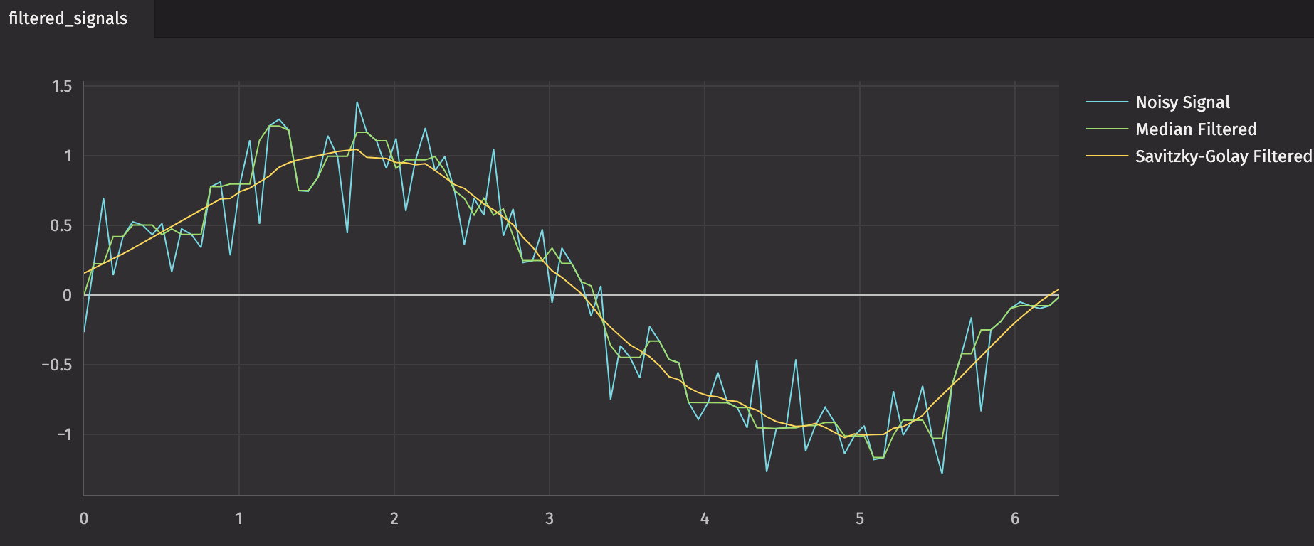
In this example, we'll generate a Sine wave and add noise. Then, we'll apply filters to reduce the noise.

from scipy.signal import medfilt, savgol_filter
import numpy as np

x = np.linspace(0, 2 * np.pi, 101)

noisy_sine_wave = np.sin(x) + np.random.normal(0, 0.25, 101)

median_filtered = medfilt(noisy_sine_wave)
savgol_filtered = savgol_filter(noisy_sine_wave, 27, 3)

The above example can be extended to use deephaven.learn in a couple of ways.

from deephaven.plot.figure import Figure
from deephaven.learn import gather
from deephaven import empty_table
from deephaven import learn
from scipy.signal import medfilt, savgol_filter
import numpy as np


def create_noisy_sine_wave(x) -> np.double:
    return np.sin(x) + np.random.normal(0, 0.25)


source = empty_table(101).update(
    formulas=[
        "X = i * (2 * Math.PI) / 100",
        "Noisy_Sine_Wave = create_noisy_sine_wave(X)",
    ]
)


def apply_median_filter(signal):
    return medfilt(signal)


def apply_savgol_filter(signal):
    return savgol_filter(signal, 27, 3)


def table_to_numpy(rows, cols):
    return np.squeeze(gather.table_to_numpy_2d(rows, cols, np_type=np.double))


def numpy_to_table(data, idx):
    return data[idx]


median_filtered = learn.learn(
    table=source,
    model_func=apply_median_filter,
    inputs=[learn.Input("Noisy_Sine_Wave", table_to_numpy)],
    outputs=[learn.Output("Median_Filtered", numpy_to_table, "double")],
    batch_size=source.size,
)

savitzky_golay_filtered = learn.learn(
    table=source,
    model_func=apply_savgol_filter,
    inputs=[learn.Input("Noisy_Sine_Wave", table_to_numpy)],
    outputs=[learn.Output("Savitzky_Golay_Filtered", numpy_to_table, "double")],
    batch_size=source.size,
)

plt = (
    Figure()
    .plot_xy(series_name="Noisy Signal", t=source, x="X", y="Noisy_Sine_Wave")
    .plot_xy(
        series_name="Median Filtered", t=median_filtered, x="X", y="Median_Filtered"
    )
    .plot_xy(
        series_name="Savitzky-Golay Filtered",
        t=savitzky_golay_filtered,
        x="X",
        y="Savitzky_Golay_Filtered",
    )
    .show()
)

Compute the nearest neighbor of every point in a set

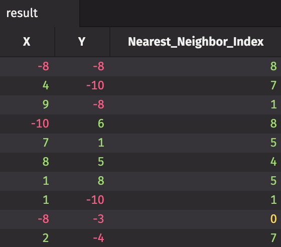
In this example, we'll use a K-d tree to compute the nearest neighbor of every point in a set. SciPy's implementation is called scipy.spatial.KDTree. We construct a two-dimensional data set with a few points, and we'll find the index of each point's nearest neighbor in the set.

from scipy.spatial import KDTree as kdtree
import numpy as np

x = np.random.randint(-10, 10, 10)
y = np.random.randint(-10, 10, 10)

data = np.vstack((x, y)).T

print(data)

tree = kdtree(data)

distances, indices = tree.query(data, k=2)

nearest_neighbor_indices = indices[:, 1]

print(nearest_neighbor_indices)

Computing the nearest-neighbor distances and indices can also be done using deephaven.learn.

from deephaven.pandas import to_table
from deephaven.learn import gather
from deephaven import learn

from scipy.spatial import KDTree as kdtree
import pandas as pd
import numpy as np

indices = np.arange(10)
x = np.random.randint(-10, 10, 10)
y = np.random.randint(-10, 10, 10)

source = to_table(pd.DataFrame({"Index": indices, "X": x, "Y": y}))


def calculate_nearest_neighbor_indices(data):
    tree = kdtree(data)
    distances, indices = tree.query(data, k=2)
    return indices[:, 1]


def table_to_numpy(rows, cols):
    return gather.table_to_numpy_2d(rows, cols, np_type=np.int_)


def numpy_to_table(data, idx):
    return data[idx]


result = learn.learn(
    table=source,
    model_func=calculate_nearest_neighbor_indices,
    inputs=[learn.Input(["X", "Y"], table_to_numpy)],
    outputs=[learn.Output("Nearest_Neighbor_Index", numpy_to_table, "int")],
    batch_size=source.size(),
)

Compute distances of various metrics between two vectors

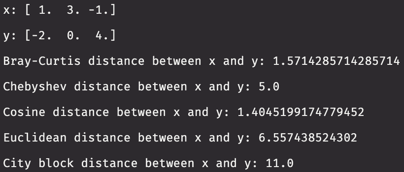
In this example, we create two three-dimensional vectors. We then compute the distance between the two vectors using metrics supported by scipy.spatial.distance.

from scipy.spatial import distance
import numpy as np

x = np.array([1, 3, -1])
y = np.array([-2, 0, 4])


def print_distances(x, y):
    print("x: " + str(x))
    print("y: " + str(y))
    print("Bray-Curtis distance between x and y: " + str(distance.braycurtis(x, y)))
    print("Chebyshev distance between x and y: " + str(distance.chebyshev(x, y)))
    print("Cosine distance between x and y: " + str(distance.cosine(x, y)))
    print("Euclidean distance between x and y: " + str(distance.euclidean(x, y)))
    print("City block distance between x and y: " + str(distance.cityblock(x, y)))


print_distances(x, y)

We can once again use deephaven.learn to calculate these distances.

from deephaven import new_table, learn
from deephaven.column import int_col
from deephaven.learn import gather

from scipy.spatial import distance
import numpy as np

source = new_table([int_col("X", [1, 3, -1]), int_col("Y", [-2, 0, 4])])


def table_to_numpy(rows, cols):
    return np.squeeze(gather.table_to_numpy_2d(rows, cols, np_type=np.intc))


def numpy_to_table(data, idx):
    return data[idx]


def print_distances(data):
    x = data[:, 0]
    y = data[:, 1]
    print("x: " + str(x))
    print("y: " + str(y))
    print("Bray-Curtis distance between x and y: " + str(distance.braycurtis(x, y)))
    print("Chebyshev distance between x and y: " + str(distance.chebyshev(x, y)))
    print("Cosine distance between x and y: " + str(distance.cosine(x, y)))
    print("Euclidean distance between x and y: " + str(distance.euclidean(x, y)))
    print("City block distance between x and y: " + str(distance.cityblock(x, y)))


learn.learn(
    table=source,
    model_func=print_distances,
    inputs=[learn.Input(["X", "Y"], table_to_numpy)],
    outputs=None,
    batch_size=source.size(),
)

Appendix: Sub-packages of SciPy

Here is a comprehensive list of the sub-packages available in SciPy, and a brief description of what each one does:

Sub-package name	Description
cluster	Clustering routines
constants	A collection of constants and conversion utilities
fft	Fourier transform methods
fftpack	Deprecated legacy Fourier transform methods
ingegrate	Numerical integration algorithms
interpolate	Tools for data interpolation
io	Data I/O
linalg	Linear algebra routines
misc	Extra miscellaneous utilities
ndimage	Image processing library
odr	Orthogonal distance regression library
optimize	Algorithms for optimizing code
signal	Signal processing routines
sparse	Tools for sparse matrix creation, handling, and procesing
spatial	Spatial structure processing algorithms
special	Special functions
stats	Statistical function library
weave	Deprecated legacy C/C++ code writing tool

Each is described below. We skip fftpack and weave because they are deprecated.## Appendix

scipy.cluster

scipy.cluster is split into two further sub-modules:

• scipy.cluster.vq supports vector quantization and K-means algorithms.
• scipy.cluster.heirarchy provides hierarchical and agglomerative clustering.

scipy.constants

scipy.constants provides an extensive number of mathematical and physical constants including (but not limited to) pi, the golden ratio, the Planck constant, subatomic particle masses, SI prefixes, binary prefixes, and many others. The full list of constants is far, far too long to include here.

scipy.fft

scipy.fft contains methods that apply the forward and reverse discrete Fourier, Sine, Cosine, and Hankel transformations to input data in N dimensions.

scipy.integrate

scipy.integrate contains a slew of methods to calculate integrals and solutions for differential equations.

scipy.interpolate

scipy.interpolate is a sub-package for objects used in data interpolation. It provides univariate and multivariate interpolation techniques, and spline interpolators.

scipy.io

scipy.io provides utilities to read and write data to and from various file formats including MATLAB, Fortran, WAV, and others.

scipy.linalg

scipy.linalg is a library of linear algebra functions. You can use this sub-module to solve eigenvalue problems, perform matrix decompositions, solve matrix equations, and construct special matrices among other things. Matrices constructed using this sub-package are of type numpy.ndarray.

This sub-module contains two further sub-packages for low-level routines: scipy.linalg.blas and scipy.linalg.lapack. These two sub-packages provide low-level functions from the Basic Linear Algebra Subprograms (BLAS) and Linear Algebra Package (LAPACK) libraries. Cython implementations of these low-level libraries exist as well.

Additionally, it provides routines for interpolative matrix decomposition via scipy.linalg.interpolative.

scipy.misc

The miscellaneous routines sub-module, scipy.misc, is the home of some example data sets and two special derivative calculators.

scipy.ndimage

scipy.ndimage contains a library of methods to perform image processing. Methods include filters, interpolation routines, measurements, and morphology routines.

scipy.odr

scipy.odr contains routines to perform orthogonal distance regression (ODR) on input data. ODR extends least squares fitting, which generally results in more accuracy in fitted curves.

scipy.optimize

The scipy.optimize sub-module provides univariate and multivariate optimization routines. These optimization routines will minimize or maximize objective functions, and can handle constraints on said functions. Solvers for both linear and nonlinear problems is supported.

There are underlying C functions for four different root finders that can be accessed via Cython.

scipy.signal

scipy.signal is SciPy's signal processing sub-module. It supports convolutions, B-splines, filters, filter designing routines, continuous time linear systems, discrete time linear systems, waveform generators, window functions, wavelet generators, maxima/minima finers, and spectral analyzers.

scipy.sparse

scipy.sparse contains functions for building and identifying sparse matrices in various formats. Additionally, it contains sparse matrix classes for each individual sparse matrix format.

This sub-module contains two sub-packages: scipy.sparse.csgraph and scipy.sparse.linalg. The first contains a library of compressed sparse graph routines, and the second contains a library of sparse linear algebra routines.

scipy.spatial

scipy.spatial contains spatial algorithms and data structures. Features include nearest-neighbor query routines, triangulation, convex hulls, Voronoi diagrams, and plotting helpers.

One sub-package of scipy.spatial is scipy.spatial.distance, which provides utilities for computing distance matrices, cheing their validity, and distance functions in numeric and boolean vectors.

There is another sub-pacakage within scipy.spatial called scipy.spatial.transform, which provides functions for spatial transformations including rotations, spherical linear interpolations of rotations, and rotation splines.

scipy.special

SciPy special functions are defined in scipy.special, which are extended to Cython via scipy.special.cython_special. Special functions include (but are not limited to) Airy, Bessel, Struve, Legendre, and statistical distributions.

scipy.stats

The sub-module, scipy.stats, contains probability distributions, summary statistics, frequency statistics, and functions for calculating correlations between distributions among other things. Methods exist for continuous, discrete, and multivariate distributions. There are are also some summary methods that can be used to describe data with little prior knowledge.

There are two sub-packages within scipy.stats: scipy.stats.mstats and scipy.stats.qmc. The former is used for calculating statistics on masked arrays, and the latter is used for describing quasi-Monte Carlo capabilities.

Related documentation

• How to use deephaven.learn
• How to use NumPy
• How to use pandas
• How to use variables and functions in query strings
• How to write a Python function
• empty_table
• User-Defined Functions
• new_table