Deephaven IDE

This guide walks through the basic Deephaven query functions and the primary components of the Deephaven IDE to create a Persistent Query.

Log in

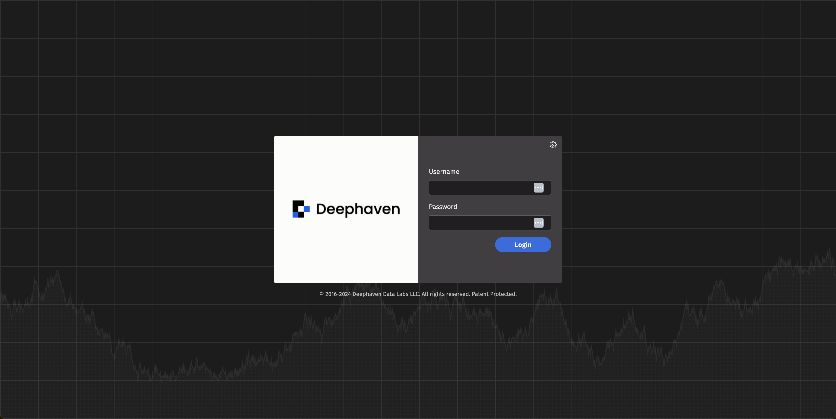
Contact your administrator to obtain the URL for your Deephaven instance and to ensure your user account is set up. By default, the URL is https://my-fqdn.com:8123/iriside, or https://my-fqdn.com:8000/iriside if Envoy is installed. Keep in mind that the port number is configurable and may vary based on your administrator's settings.

Once you navigate to your URL, you should see a screen similar to the following:

Code Studio

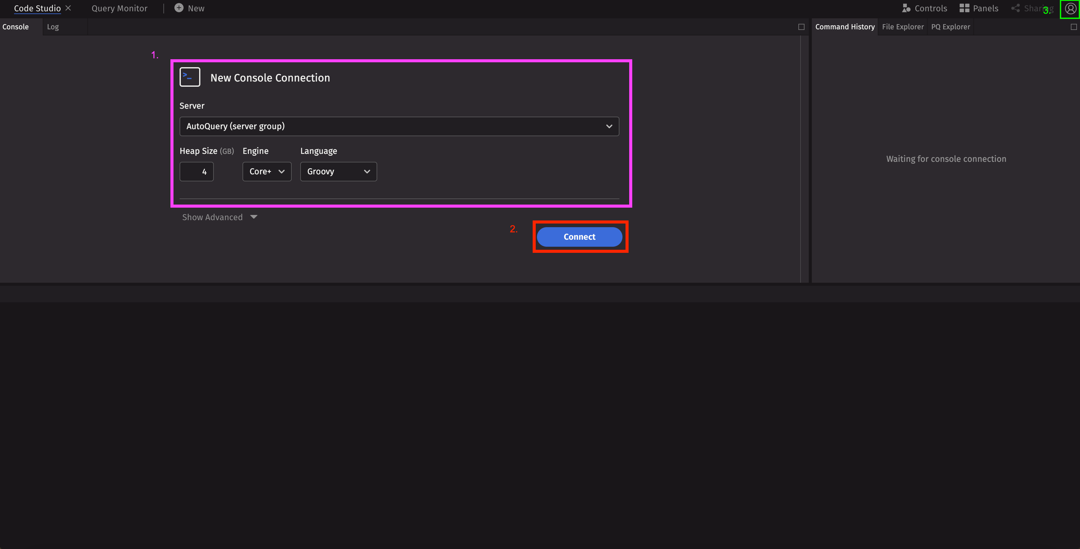
The first thing you will see after logging in as a new user is the Code Studio and a prompt to create a New Console Connection. Once the Code Studio is connected to a server, you can quickly develop and prototype queries.

1. Worker configuration

   In this section, you can configure the type of worker to use. Choose the server to run on, the amount of heap, the engine (Legacy or Core+), and the language in which you would like to develop. There is also an Advanced section with additional parameters, but we won't cover that here.

2. Connect to a worker

   Click the Connect button to launch a new Deephaven worker

3. Customize the IDE

   Click the gear icon to access a menu with options to personalize your Deephaven experience or log out.

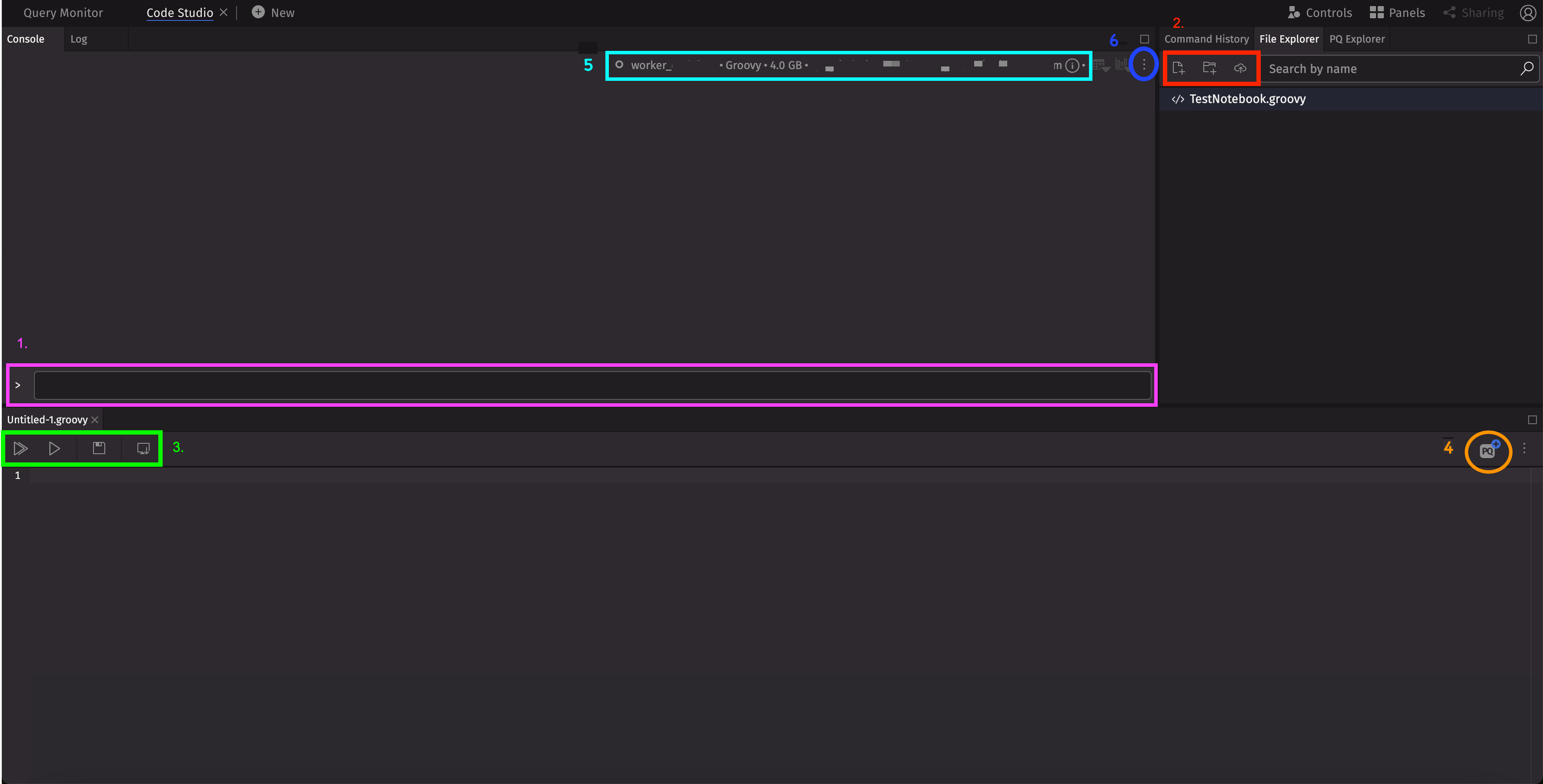
For now, leave the default parameters and connect to the new query worker. Once connected, your screen should look like this:

1. Execute commands

   This field allows you to write and execute Deephaven commands.

2. Create new Notebooks

   From the File Explorer, you can create new notebooks and folders, or import notebooks.

3. Manage Notebooks

   From the Notebook toolbar, you run the whole notebook or a section of it, save your script, or download it.

4. Save PQ

   Save your notebook as a Persistent Query.

5. Worker Information

   This section displays information about your worker. Hover over the info icon to see more.

6. Console Menu

   Use this menu to restart or disconnect your worker.

Develop a Persistent Query

Persistent Queries are one of the core building blocks of a Deephaven system. Once deployed, they continuously run on a schedule and can be connected to dashboards, external applications, or even other Persistent Queries.

Access data

There are many ways to retrieve data from a Deephaven worker; below are just a few examples.

Upload a CSV

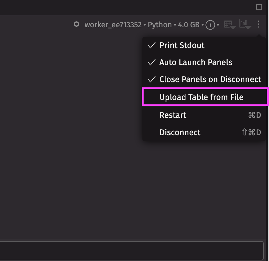
The simplest method is to upload a CSV. In the console menu, select Upload Table from File and upload the CSV of your choice.

Query historical data

The historical table API, db.historical_table("{NAMESPACE}", "{TABLE_NAME}"), is used to query static data that has already been imported into the system, such as the LearnDeephaven tables, which can be optionally installed with your deployment. The examples in this crash course use the LearnDeephaven.StockQuotes table.

Query live data

The live table API, db.live_table("{NAMESPACE}", "{TABLE_NAME}"), queries a streaming table in real time. The stream must be set up by a developer, such as the internal tables in the DbInternal namespace. These tables come with the system and contain worker logs, performance data, and other metrics.

Filter data

When querying any table, it is good practice to filter so you are not pulling in more data than you can handle.

t = db.historicalTable("LearnDeephaven", "StockQuotes").where("Date = `2017-08-25`")

t = db.historical_table("LearnDeephaven", "StockQuotes").where("Date = `2017-08-25`")

Other ways to filter include:

• where_in
• where_not_in
• where_one_of
• head
• tail
• slice
• head-pct
• tail_pct
• slice_pct

Manipulate data columns

Once you have data to work with, you may want to transform your columns or create new ones. The main functions for column manipulation are view, select, update_view, and update.

t = db.historicalTable("LearnDeephaven", "StockQuotes")
  .where("Date = `2017-08-25`")

// View only displays the columns inputted. Values are calculated as needed.
tV = t.view("Date", "USym", "Bid", "Ask", "Mid=(Bid+Ask)/2")

// Select does the same thing, but values are calculated right away and put into memory.
tS = t.select("Date", "USym", "Bid", "Ask", "Mid=(Bid+Ask)/2")

// UpdateView creates a new column, but retains the current columns. Values are calculated as needed.
tUv = t.updateView("Mid=(Bid+Ask)/2")

// Update does the same, but values are calculated right away and put into memory.
tU = t.update("Mid=(Bid+Ask)/2")

t = db.historical_table("LearnDeephaven", "StockQuotes").where("Date = `2017-08-25`")

# View only displays the columns inputted. Values are calculated as needed.
t_v = t.view(["Date", "USym", "Bid", "Ask", "Mid=(Bid+Ask)/2"])

# Select does the same thing, but values are calculated right away and put into memory.
t_s = t.select("Mid=(Bid+Ask)/2")

# Update_view creates a new column, but retain the current columns. Values are calculated as needed.
t_uv = t.update_view("Mid=(Bid+Ask)/2")

# Update does the same, but values are calculated right away and put into memory.
t_u = t.update("Mid=(Bid+Ask)/2")

Other ways to manipulate columns include:

• lazy_update
• sort
• drop_columns
• rename_columns
• move_columns
• rename_columns

Aggregate data

Deephaven comes with many built-in aggregations.

t = db.historicalTable("LearnDeephaven", "StockQuotes")
  .where("Date = `2017-08-25`")

tSum = t.view("Date", "USym", "BidSize").sumBy("Date", "USym")

t = db.historical_table("LearnDeephaven", "StockQuotes").where("Date = `2017-08-25`")

t_sum_by = t.view(["Date", "USym", "BidSize"]).sumBy(["Date", "USym"])

This example uses multiple aggregations to create new columns that are the average and the standard deviation of the Bid column, keyed by the Exchange and USym:

import static io.deephaven.api.agg.Aggregation.AggAvg
import static io.deephaven.api.agg.Aggregation.AggStd

t = db.historicalTable("LearnDeephaven", "StockQuotes")
  .where("Date = `2017-08-25`")

tAgg = t.aggBy(
      [AggAvg("AvgBidPrice=Bid"), AggStd("StdBidPrice=Bid")],
      "Exchange", "USym",
)

from deephaven import agg

t = db.historical_table("LearnDeephaven", "StockQuotes").where("Date = `2017-08-25`")

tAgg = t.agg_by(
    [agg.avg("AvgBidPrice=Bid"), agg.std("StdBidPrice=Bid")], by=["Exchange", "USym"]
)

The agg_by reference page provides a full list of aggregations.

Join data

There are several ways to join data, but the most basic is Deephaven's natural_join, which functions like SQL's LEFT JOIN.

This example joins the column BidSize from our t_sum table from earlier onto the original table, creating a new column called BidSizeSum:

t = db.historicalTable("LearnDeephaven", "StockQuotes")
  .where("Date = `2017-08-25`")

tSum = t.view("Date", "USym", "BidSize").sumBy("Date", "USym")

tJoined = t.naturalJoin(tSum, "Date,USym", "BidSizeSum=BidSize")

t = db.historical_table("LearnDeephaven", "StockQuotes").where("Date = `2017-08-25`")

t_sum = t.view(["Date", "USym", "BidSize"]).sum_by(["Date", "USym"])

t_joined = t.natural_join(t_sum, "Date,USym", "BidSizeSum=BidSize")

Other available joins include:

• aj
• exact_join
• full_outer_join
• join
• left_outer_join
• multi_join
• raj
• range_join

Plot data

Deephaven has a built-in plotting library.

t = db.historicalTable("LearnDeephaven", "StockQuotes")
  .where("Date = `2017-08-25`")

// Filter for USym, Exchange and timestamps within open hours
applArcaPrices = t.where("USym = `AAPL`", "Exchange = `Arca`", "inRange(Timestamp, '2017-08-25T09:30:00 ET', '2017-08-25T16:00:00 ET')")

// Plot your data
myPlot = plot("AAPL Prices",  applArcaPrices, "Timestamp", "Bid")
    .chartTitle("AAPL Arca During Open")
    .show()

from deephaven.plot.figure import Figure

t = db.historical_table("LearnDeephaven", "StockQuotes").where("Date = `2017-08-25`")

# Filter for USym, Exchange and timestamps within open hours
appl_arca_prices = t.where(
    [
        "USym = `AAPL`",
        "Exchange = `Arca`",
        "inRange(Timestamp, '2017-08-25T09:30:00 ET', '2017-08-25T16:00:00 ET')",
    ]
)

# Plot your data
my_plot = (
    Figure()
    .figure_title("AAPL Arca During Open")
    .plot_xy(
        series_name="AAPL Prices",
        t=appl_arca_prices,
        x="Timestamp",
        y="Bid",
    )
    .show()
)

Other ways to plot data include:

• Deephaven + Plotly express
• Matplotlib and Seaborn
• Deephaven plotting via the UI

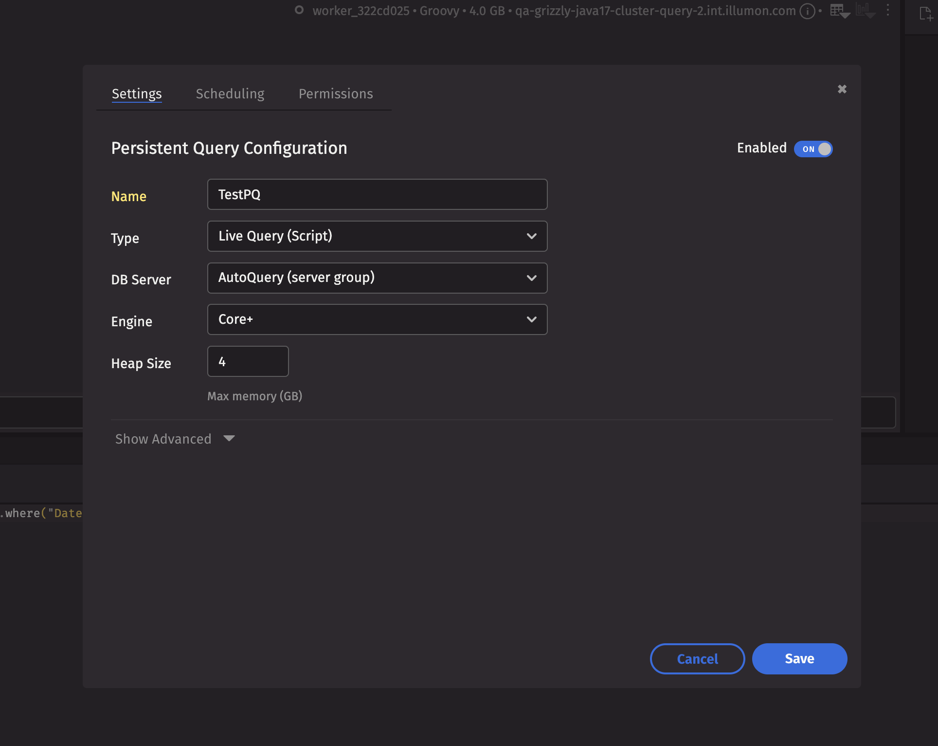
Deploy your code as a Persistent Query

Copy the code from the plotting example into a notebook. The PQ+ button at the top right of the Notebook window opens a Persistent Query (PQ) configuration screen. Name your PQ whatever you want, leave the rest as their default values, and hit the Save button.

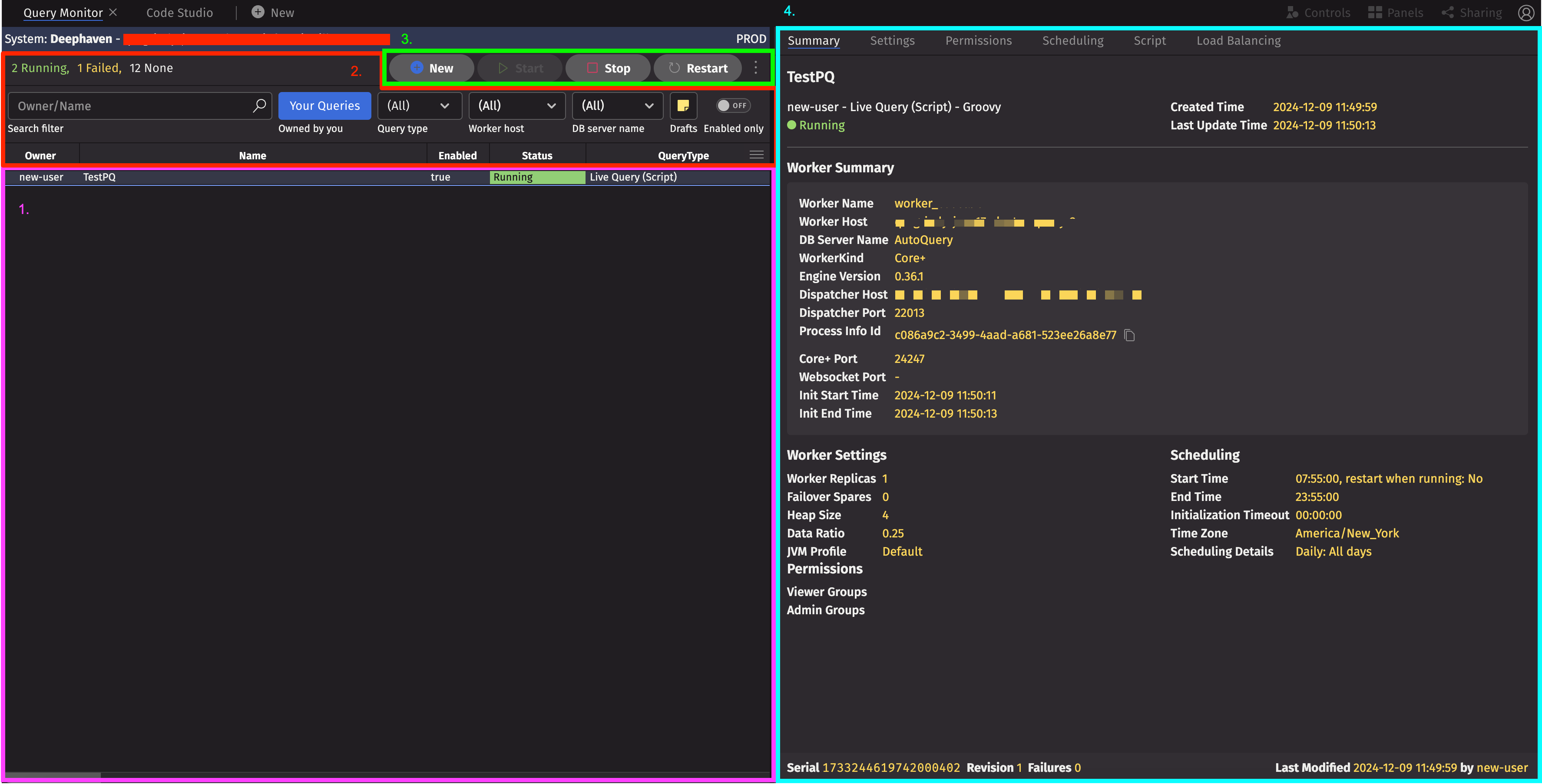
Query Monitor

When you deploy a PQ, you should see it in the Query Monitor. It can be accessed next to the Code Studio tab at the top of your IDE. The Query Monitor is a GUI for managing any PQs you have access to.

1. PQ Table

   Here is where you'll see a table of PQs, their statuses, and other information.

2. PQ Filter

   These data filters narrow down your information and help you find the PQ(s) you are searching for.

3. PQ Control Buttons

   These buttons provide options to create a new PQ or start/stop/restart the selected PQ right from the Query Monitor.

4. PQ Config

   The Summary window provides additional details about the selected PQ and other tabs to modify its configuration.

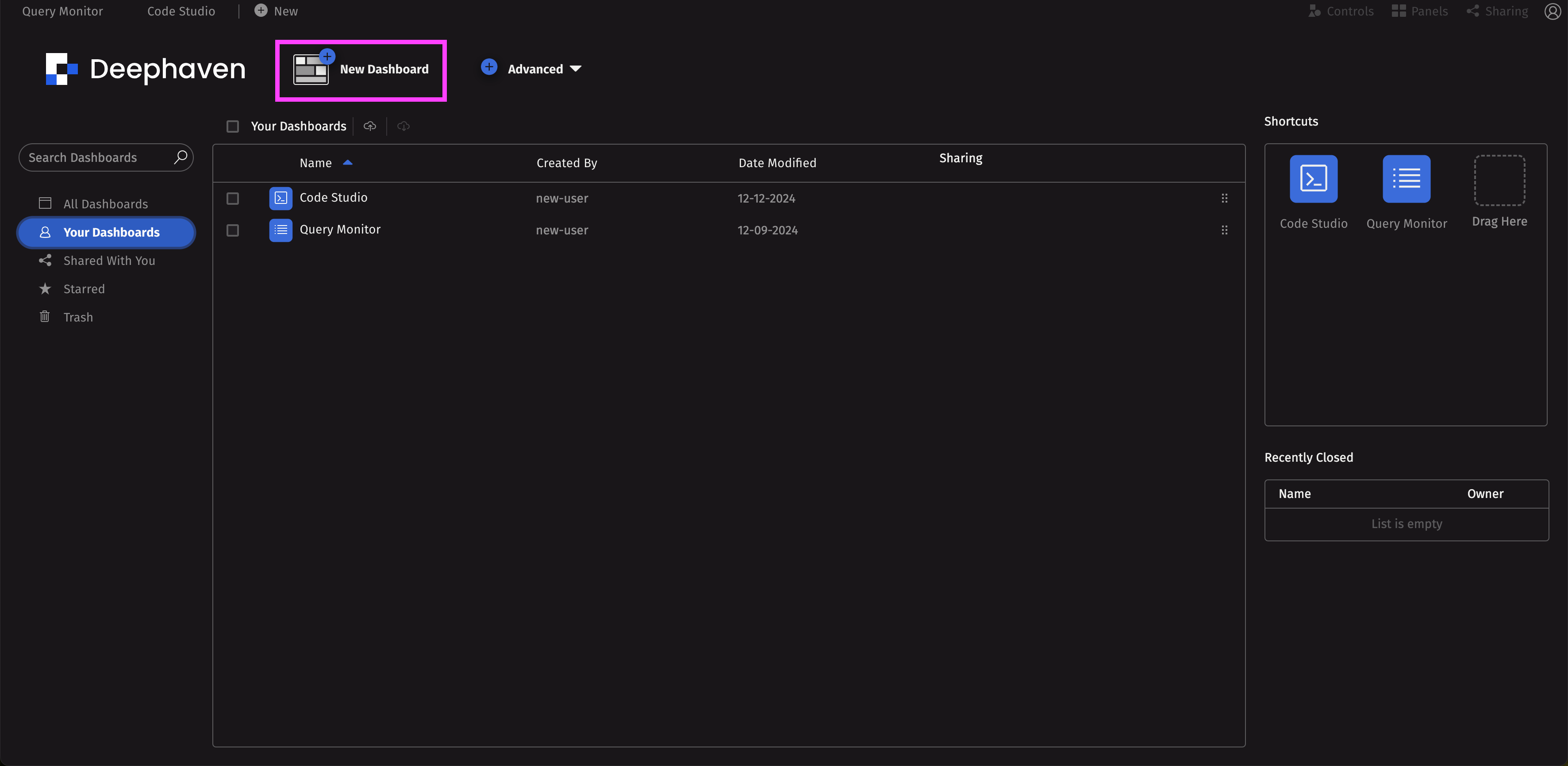
Create a dashboard

Once your PQ is deployed and running, you can create a dashboard to display its components and share it with others. Click on the +New icon near the Code Studio tab to create a new dashboard.

Once you start a fresh dashboard, navigate to the Panels drop-down in the top right, search for your PQ, and drop in whatever components you would like.

You should see an entry for your dashboard on the previous screen where you can share it with other Deephaven users.

What's Next?

Learn how to develop scripts using Visual Studio.

Related documentation

• Query Monitor
• Code Studio
• Create a dashboard by hand
• Use filters
• Use select, view, and update
• Multi-aggregation
• Exact and relational joins
• Work with plots