Pipeline and multi-thread your workload

Depending on your use case, Deephaven provides several methods of scaling your queries. There are two main dimensions along which to increase the resources available to your query: you may pipeline the query, where you divide it into several stages, or you may shard the query, where you divide it into independent units of work and then combine those results.

Pipeline Your Workload

Pipelining a query allows you to increase the computational resources available, either across JVMs or even across machines in a cluster. Moreover, downstream consumers can often share the results of a pipeline stage, reducing the overall computation required.

To pipeline a query, you must first determine sensible boundaries between query stages. An example of a useful pipeline stage may be part of the query that summarizes its input data, or transforms one stream into another similarly sized stream. If you divide the query without proper consideration for the communications overhead between the constituent parts of the query you may end up with slower processing than you started with.

The two primary methods of pipelining a query in Deephaven are:

1. Feeding intermediate results into a persistent table, e.g., via binary logs ingested at the Data Import Server or embedding a Data Import Server in your Persistent Query.
2. Sending the current state of intermediate results to another worker via Barrage.

Persistent tables

Persistent tables are a good solution when input data is transformed into a derived stream for which the history may be useful. For example, you may want to downsample incoming quotes or trades into 1-minute bins. The worker running your downsampling process can write out new streams that are then imported via the DataImportServer and used by other queries. Similarly, when performing complex computation such as option fitting, you may gather many inputs and then write out binary logs for downstream queries to consume.

See our how-to guide on the System Table Logger for more information on streaming data to a System Table with binary logs. You may also structure your query to embed a Data Import Server using the Derived Table Writer. The choice between a system table logger and a derived table writer depends on your use case. Binary logs have a lower initial setup cost; you must create a schema, but no data routing configuration or explicit storage configuration is necessary.

An embedded DIS, on the other hand, requires storage and routing configuration, but does have some advantages over binary logs. Namely:

• There is no need for intermediate binary log files, which reduces overall storage requirements.
• A DIS can provide exactly-once delivery, and the persistent state of a table can be used to resume processing from where the query left off.

Because the Derived Table Writer requires storage configuration, it must execute on the same query node each time it is restarted. You cannot use automatic server selection to select the query server. In contrast, using a system table logger requires no storage configuration. Binary logs are written to a standard path (typically /var/log/deephaven/binlogs) and the tailer sends them to the appropriate DIS. The query itself never reads existing binary logs, therefore the server selection provider can select any node in the cluster to execute a query using the system table logger.

Barrage Tables

Barrage tables are a good solution for pipelining your query when you care about a smaller current state, as compared to the entire input stream. For example, you may have one query compute the most current market data or firmwide positions and then make those results available to other queries.

Barrage tables utilize gRPC connections to consistently replicate data across JVM boundaries. A Barrage table requires more memory on both the subscriber and producer than a persistent table. The subscriber must hold the entire table in memory. When a consumer is subscribing, the producer must also have sufficient memory to generate a consistent snapshot of the complete table to send to the subscriber.

For more information on sharing tables with Barrage see Sharing tables with Groovy or Sharing tables with Python.

Employ multithreading

The other alternative to parallelizing your query is to shard it. In sharding, you divide the workload into disjoint sets. You may shard a query across multiple JVMs or within a single JVM. Sharding across multiple JVMs gives your workload the most independence possible, but is more likely to result in duplicated work, and combining the results is more expensive than if all the intermediate results are in the same JVM.

A Deephaven query operation can be divided into two phases. In the first phase, the query operation is initialized. After a query operation is initialized, the results are updated as part of the Update Graph refresh cycle. When you initialize a query operation, the initial state of the result is computed before the call returns. Some calls (notably select, update, and where) may internally parallelize the operation further by dividing a table into segments and working on distinct segments in threads before combining the results.

If the data can be divided into independent partitions, then each operation can be processed in parallel, either manually or by primitives that Deephaven provides. In particular, a Partitioned Table automatically parallelizes initialization for each constituent. When a PartitionedTable transforms tables (either through the transform method or with a proxy), it uses Deephaven's update method under the hood - naturally parallelizing the computation across the constituent tables. By default, a worker uses as many threads as there are CPUs. This can be controlled by changing the OperationInitializationThreadPool.threads configuration property.

The UpdateGraphProcessor also uses as many threads as there are CPUs by default (controllable with the PeriodicUpdateGraph.updateThreads configuration property). For operations that internally parallelize (like select, update, and where), multiple threads can be used for a single operation. Otherwise, tables that have no dependencies are updated in parallel. As each constituent of a PartitionedTable table is independent, using a Proxy or transform permits each constituent to be updated in parallel with the other constituents.

Dividing data with a where() clause

The first step of sharding a query is to divide the source data. This can be accomplished using a where() clause to filter out undesirable data. For example, if you have four separate remote query processors, each processing one-fourth of the universe, you may preface your query with a clause like .where(“Symbol.hashCode() % 4 == QUERY_PARTITION_NUMBER”), and then set the QUERY_PARTITION_NUMBER in your QueryScope.

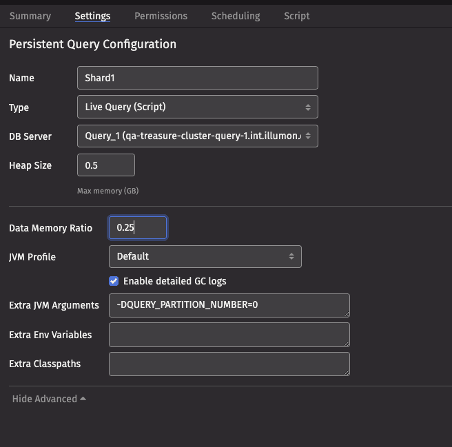
One effective way of setting a QueryScope parameter is to use JVM system properties added to your extra JVM arguments in the query configuration. For example, in the following script, the QUERY_PARTITION_NUMBER is read from the system property and stored in a variable in the Groovy binding. Each shard of the query can use the same code, with only the query’s configuration changing the behavior.

QUERY_PARTITION_NUMBER=Integer.parseInt(System.getProperty("QUERY_PARTITION_NUMBER"))
t=db.liveTable("FeedOS", "EquityQuoteL1").where("Date=today()").renameColumns("Symbol=LocalCodeStr").where("abs(Symbol.hashCode()) % 4 == QUERY_PARTITION_NUMBER")
symbols=t.selectDistinct("Symbol")

A Java property can also be retrieved from Python:

import jpy

javaSystem = jpy.get_type("java.lang.System")
javaSystem.getProperty("QUERY_PARTITION_NUMBER")
QUERY_PARTITION_NUMBER = int(javaSystem.getProperty("QUERY_PARTITION_NUMBER"))

t = (
    db.live_table("FeedOS", "EquityQuoteL1")
    .where("Date=today()")
    .rename_columns("Symbol=LocalCodeStr")
    .where("abs(Symbol.hashCode()) % 4 == QUERY_PARTITION_NUMBER")
)
symbols = t.select_distinct("Symbol")

The advanced options of the Settings panel in the Query Monitor allow you to set system properties:

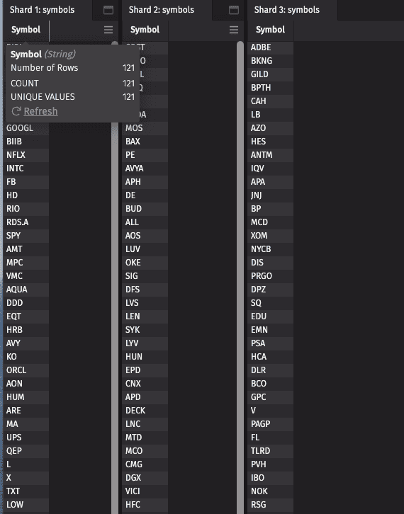
Each query will have a disjoint set of symbols in the table “Symbol”:

where clauses are an effective technique when your data is not already naturally partitioned, and you are operating the query in distinct JVMs. Each input row is processed in each JVM, but the only additional state that must be maintained is the row set that identifies the responsive rows for downstream operations. Each JVM must read the entire data set for columns required to execute the where() clause, and very likely must read the complete raw binary data for other columns as well. This is because Deephaven stores its columns in pages and if the data set is uniformly distributed within the pages, you will likely require at least one row from each page. Downstream operations need not examine each cell, but the unused data still requires memory and network or disk resources.

Fetching a specific internal partition

If the data is already naturally partitioned, you may be able to use those partitions for your parallelization. For live tables, the Deephaven system has two partitioning columns. The column partition, often Date is visible in the schema. The internal partition is not visible in the schema, and is used to separate streams that come from distinct sources. You can add a column for the internal partition to the liveTable or historicalTable call using a TableOptions.Builder:

import io.deephaven.enterprise.database.TableOptions

with_internal_partition=db.liveTable("FeedOS", "EquityQuoteL1", TableOptions.newLiveBuilder().internalPartitionColumn("InternalPartition").build())

Similarly, in Python you can pass the internal_partition_column argument to live_table and historical_table:

with_internal_partition = db.live_table(
    "FeedOS", "EquityQuoteL1", internal_partition_column="InternalPartition"
)

After adding an internal partition column, it can be used in subsequent query operations. For example, you may use select_distinct to retrieve a list of the available partitions, and then use where to filter the data to a subset of partitions for each shard. Like other partitioning columns, the internal partitioning column automatically has a Data Index, which avoids the need to read the full data set. If you interject query operations between fetching the table and using the internal partitioning column, then you lose the performance benefits of the Data Index.

Care must be taken at the data sources to use internal partitioning to shard your query. In particular, for queries that combine data sources, you should ensure that the internal partitioning is consistent among the data sources. When the partitioning is not consistent, you should select the source that drives the queries' performance and then use that source’s natural partitioning. The other data sources must then be filtered (across all relevant partitions) to match the primary data source’s partitioning scheme.

Partitioned tables

The Deephaven API is centered on the Table. A partitioned table is a Table that contains other Tables. Using a partitioned table allows you to divide a table into segments. The two most common ways of creating a partitioned table:

1. Dividing the table using the value of a column using the partition_by from Python or partitionBy from Groovy.
2. Requesting a partitioned table from the Database object using live_partitioned_table or historical_partitioned_table from Python. Similarly, the Groovy Database object provides livePartitionedTable and historicalPartitionedTable methods.

partitionBy

For example, to divide the table t by the USym and Expiry columns, you could call t.partitionBy("USym", "Expiry"). The partitionBy call has the advantage over the equivalent iterative where clauses in that the USym and Expiry columns need only be evaluated once, no matter how many combinations of keys and values exist. Moreover, the set of possible keys need not be known in advance; the partitionedTable interface provides the ability to listen for newly created keys or key-Table pairs.

A simple way of partitioning a Table is to use the hashCode of your query’s partitioning key. For example, you could divide each of your source tables by the hashCode of USym:

import io.deephaven.configuration.Configuration
N_PARTITIONS = Configuration.getInstance().getIntegerWithDefault("N_PARTITIONS", 4)
marketDataPartitioned = marketDataSource.updateView("Partition=abs(Symbol.hashCode()) % N_PARTITIONS").partitionBy("Partition")

import jpy

Configuration = jpy.get_type("io.deephaven.configuration.Configuration")
N_PARTITIONS = Configuration.getInstance().getIntegerWithDefault("N_PARTITIONS", 4)
market_data_partitioned = market_data_source.update_view(
    "Partition=abs(LocalCodeStr.hashCode()) % N_PARTITIONS"
).partition_by("Partition")

The Deephaven engine processes the partitionBy operation with a single thread, but once the partitionBy operation creates the independent tables, downstream operations can make use of threads.

The partitionBy method requires generating a group of data for each constituent table. In some circumstances, this grouping operation can be almost as expensive as the underlying operation to parallelize. For example, to simply count the number of values by a key, the bulk of the operation is creating a grouping. As the partitionBy is a fundamentally single-threaded operation, simply performing the count operation with a single thread would be less expensive than dividing the work into multiple threads.

livePartionedTable and historicalPartitionedTable

When requesting a Table from the Deephaven database object (db in your script), normally, you call liveTable or historicalTable. These methods retrieve a single table that can represent many partitions of data (e.g., years worth of date partitions for a historical table or all of the available internal partitions for a given date). To limit the data, best practice is to begin with a partition filter. For example, to retrieve the ProcessEventLog for today:

pel=db.liveTable("DbInternal", "ProcessEventLog").where("Date=today()")

pel = db.live_table("DbInternal", "ProcessEventLog").where("Date=today()")

Instead of retrieving all of the partitions as a single table, they can be retrieved as a partitioned table:

pel_pt=db.livePartitionedTable("DbInternal", "ProcessEventLog")

pel_pt = db.live_partitioned_table("DbInternal", "ProcessEventLog")

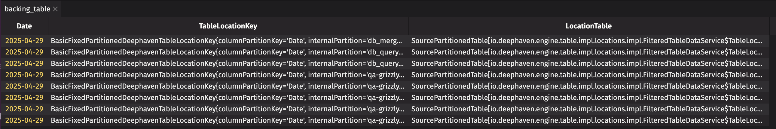
The table method retrieves the underlying Table of tables:

backing_table=pel_pt.table()

backing_table = pel_pt.table

In this example, the Date column partition is displayed together with the TableLocationKey and LocationTable columns:

The partitioned table can be filtered on the column partition as follows:

pel_pt_today=pel_pt.filter(Filter.from("Date=today()")

pel_pt_today = pel_pt.filter("Date=today()")

For example, the following query creates a TableMap of the LearnDeephaven.StockTrades table:

stockTrades=db.historicalPartitionedTable("LearnDeephaven", "StockTrades")

stock_trades = db.historical_partitioned_table("LearnDeephaven", "StockTrades")

It is important to note that the TableLocationKeys for different source tables generally do not coincide. Therefore, you can not join tables from two PartitionedTables that are derived from livePartitionedTable or historicalPartitionedTable.

PartitionedTable Proxy

To enable convenient usage, the PartitionedTable object exposes a proxy method in (Python and Groovy) that permits you to operate on the partitioned table as if it were a Table.

marketData = marketDataPartitioned.proxy()

market_data = market_data_partitioned.proxy()

The "marketData" table can now be used as if it were any other Deephaven table; for example:

withParity=marketData.updateView("parity=product.substring(12, 13)")
puts=withParity.where("parity=`P`")

with_parity = market_data.update_view(["parity=product.substring(12, 13)"])
puts = with_parity.where("parity=`P`")

The updateView and where clauses are evaluated independently on each table within the Partitioned Table, and a new PartitionedTable is created and presented as the table proxy "puts". The Partitioned Table backing "puts" has one Table pair for each table in the original Partitioned Table (even if the result of the where is a zero-sized Table). Continuing the same example, we can operate on both the original "marketData" and the "puts" tables:

calls = withParity.where("parity=`C`")
putRenames = puts.view("put_bid=bid_price", "put_ask=ask_price", "put_bid_size=bid_quantity", "put_ask_size=ask_quantity")
                .dropColumns("bid_price", "ask_price", "bid_quantity", "ask_quantity")

calls = with_parity.where("parity=`C`")
put_renames = puts.update_view(
    [
        "put_bid=bid_price",
        "put_ask=ask_price",
        "put_bid_size=bid_quantity",
        "put_ask_size=ask_quantity",
    ]
).drop_columns(["bid_price", "ask_price", "bid_quantity", "ask_quantity"])

The putRenames and calls tables are backed by partitioned tables with a parallel key set, which places each product into a consistent bucket. Therefore, we can use join operations on the putRenames and calls tables independently, as follows:

putsWithCalls = putRenames.naturalJoin(calls, "Date,product", "call_bid=bid_price,call_bid_size=bid_quantity,call_ask=ask_price,call_ask_size=ask_quantity")

puts_with_calls = put_renames.natural_join(
    calls,
    ["Date", "product"],
    [
        "call_bid=bid_price",
        "call_bid_size=bid_quantity",
        "call_ask=ask_price",
        "call_ask_size=ask_quantity",
    ],
)

Of particular note, when the proxy() method's sanityCheckJoinOperations parameter is set to true, the Deephaven engine performs additional work to verify that each join key only exists in one of the constituent tables within the PartitionedTable and that the keys are consistent between the two partitioned tables. If you are sure that the keys must be consistent, you can disable join sanity checking for improved performance and memory usage.

Transform

The PartitionedTable proxy uses transform (Java or Python) under the hood.

Transform provides more flexibility than a proxy. In particular, you are working with an actual Table instead of the proxy and therefore can use any Table member function or a static function that accepts a table. Additionally, instead of being limited to performing one operation and then creating a new PartitionedTable proxy, you can chain many operations together, eliminating unnecessary intermediate Partitioned Tables.

For example, the previous example can be combined into one transform for all of the transformations for the puts_renamed table:

import io.deephaven.util.SafeCloseable

defaultCtx = ExecutionContext.getContext()

puts_renamed = marketDataPartitioned.transform(t -> {
    try (final SafeCloseable ignored = defaultCtx.open()) {
        return t.updateView("parity=product.substring(12, 13)")
            .where("parity=`P`")
            .updateView("put_bid=bid_price", "put_ask=ask_price", "put_bid_size=bid_quantity", "put_ask_size=ask_quantity")
            .dropColumns("bid_price", "ask_price", "bid_quantity", "ask_quantity")
    }
})
```


````python test-set=1 skip-test
from deephaven.execution_context import get_exec_ctx

ctx = get_exec_ctx()


def put_function(t):
    with ctx:
        return (
            t.update_view("parity=product.substring(12, 13)")
            .where("parity=`P`")
            .update_view(
                [
                    "put_bid=bid_price",
                    "put_ask=ask_price",
                    "put_bid_size=bid_quantity",
                    "put_ask_size=ask_quantity",
                ]
            )
            .drop_columns(["bid_price", "ask_price", "bid_quantity", "ask_quantity"])
        )
puts_renamed = market_data_partitioned.transform(put_function)```

Merging results

In some cases, the partitioned table is a suitable result, and it can be exposed to other queries or to UI widgets. A partitioned table proxy result can be converted back to a PartitionedTable with the target method. To create a single Table that can be viewed by the UI, or to reaggregate results, the merge() operation should be used.

For example, if we wanted to parallelize a countBy operation across a large Table, we could perform the following operations:

marketData=db.historicalPartitionedTable("OPRA", "optionTrades")
counted = marketData.proxy().countBy("Count", "product")
merged = counted.target().merge().sumBy("product")

market_data = db.historical_partitioned_table("OPRA", "optionTrades")
counted = market_data.proxy().count_by("Count", "product")
merged = counted.target.merge().sum_by("product")

Related documentation

• Troubleshooting
• Data Import Server
• Binary logs
• Query Monitor