Rolling aggregations

This guide provides a comprehensive overview of how to use the updateBy table operation for rolling calculations and aggregations. This operation creates a new table containing columns with aggregated calculations (called UpdateByOperations) from a source table. The calculations can be cumulative, windowed by rows (ticks), or windowed by time. They can also be performed on a per-group basis, where groups are defined by one or more key columns.

For a complete list of all available UpdateByOperations that can be performed with updateBy, see the reference page.

The use of updateBy requires one or more of these calculations, as well as zero or more key columns to define groups. The resultant table contains all columns from the source table, as well as new columns if the output of the UpdateByOperation renames them. If no key columns are given, then the calculations are applied to all rows in the specified columns. If one or more key columns are given, the calculations are applied to each unique group in the key column(s).

What are rolling aggregations?

Rolling aggregations are unique from dedicated and combined aggregations for two reasons.

Preservation of data history

When performing aggregations with dedicated and combined aggregations, the output table contains a single row for each group. In contrast, rolling aggregation tables have the same number of rows as the source table. Thus, they preserve data history, whereas the others do not.

To illustrate this, consider a cumulative sum on a single grouping column with two key values. Notice how resultDedicated and resultCombined have two rows - one for each group. In contrast, resultRolling has 20 rows - one for each row in the source table. You can see how the cumulative sum increases over time in the latter case.

source = emptyTable(20).update("Key = (ii % 2 == 0) ? `A` : `B`", "Value = ii")

resultRolling = source.updateBy(CumSum("SumValue=Value"), "Key")
resultDedicated = source.sumBy("Key")
resultCombined = source.aggBy(AggSum("SumValue=Value"), "Key")

Windowing

Dedicated and combined aggregations are all cumulative. They calculate aggregated values over an entire table. In contrast, rolling aggregations can be either cumulative or windowed.

A windowed aggregation is one that only calculates aggregated values over a subset of the table. This subset is defined by a window, which can be specified in terms of rows (ticks) or time. For example, a windowed sum may calculate the aggregated sum over the previous 10 rows in the table. When a new row ticks in, the aggregated value is updated to reflect the new row and the oldest row that is no longer in the window.

To illustrate this, consider the following example, which calculates a cumulative sum and a rolling sum with updateBy. The rolling sum is applied over the previous 3 rows, so the SumValue column differs from its cumulative counterpart:

source = emptyTable(6).update("Value = ii")

result = source.updateBy([
    CumSum("CumSumValue=Value"),
    RollingSum(3, "RollingSumValue=Value")
])

Basic usage examples

The following examples demonstrate the fundamental patterns for using updateBy.

A single UpdateByOperation with no grouping columns

The following example calculates the tick-based rolling sum of the X column in the source table. No key columns are provided, so a single group exists that contains all rows of the table.

source = emptyTable(20).update("X = i")

result = source.updateBy(RollingSum(3, 0, "RollingSumX = X"))

Multiple UpdateByOperations with no grouping columns

The following example builds on the previous by performing two UpdateByOperations in a single updateBy. The cumulative minimum and maximum are calculated, and the range is derived from them.

source = emptyTable(20).update("X = randomInt(0, 25)")

result = source.updateBy([CumMin("MinX = X"), CumMax("MaxX = X")]).update("RangeX = MaxX - MinX")

Multiple UpdateByOperations with a single grouping column

The following example builds on the previous by specifying a grouping column. The grouping column is Letter, which contains alternating letters A and B. As a result, the cumulative minimum, maximum, and range are calculated on a per-letter basis. The result table is split by letter via where to show this.

source = emptyTable(20).update("Letter = (i % 2 == 0) ? `A` : `B`", "X = randomInt(0, 25)")

result = source.updateBy([CumMin("MinX = X"), CumMax("MaxX = X")], "Letter").update("RangeX = MaxX - MinX")

resultA = result.where("Letter == `A`")
resultB = result.where("Letter == `B`")

A single UpdateByOperation applied to multiple columns with multiple grouping columns

The following example builds on the previous by applying a single UpdateByOperation to multiple columns as well as specifying multiple grouping columns. The grouping columns, Letter and Truth, contain alternating letters and random true/false values. Thus, groups are defined by unique combinations of letter and boolean. The result table is split by letter and truth value to show the unique groups.

source = emptyTable(20).update("Letter = (i % 2 == 0) ? `A` : `B`", "Truth = randomBool()", "X = randomInt(0, 25)", "Y = randomInt(50, 75)")

rollingSumOps = RollingSum(5, 0, "RollingSumX = X", "RollingSumY = Y")
minOps = CumMin("MinX = X", "MinY = Y")
maxOps = CumMax("MaxX = X", "MaxY = Y")

result = source.updateBy([rollingSumOps, minOps, maxOps], "Letter", "Truth").update("RangeX = MaxX - MinX", "RangeY = MaxY - MinY")
resultATrue = result.where("Letter == `A`", "Truth == true")
resultAFalse = result.where("Letter == `A`", "Truth == false")
resultBTrue = result.where("Letter == `B`", "Truth == true")
resultBFalse = result.where("Letter == `B`", "Truth == false")

Applying an UpdateByOperation to all columns

The following example uses Fill to fill null values with the most recent previous non-null value. No columns are given to Fill, so the forward-fill is applied to all columns in the source table except for the specified key column(s). This means the original columns (e.g., X and Y) are replaced in the result table by new columns of the same name containing the forward-filled values.

source = emptyTable(10).update("Letter = (i % 2 == 0) ? `A` : `B`", "X = (i % 3 == 0) ? NULL_INT : i", "Y = (i % 5 == 2) ? i : NULL_INT")

result = source.updateBy(Fill(), "Letter")

updateBy vs updateby

This document refers to updateBy and updateby throughout. They are not identical:

• updateBy always refers to theupdateBy table operation. This is always invoked as a method on a table:

result = source.updateBy(...)

• updateby refers to the Groovy package module housing all of the functions and related plumbing. The UpdateByOperation interface contains the updateBy operations themselves, such as EmMax and RollingFormula.

This distinction will be important to keep in mind as you progress through the document.

Cumulative aggregations

Cumulative aggregations are the simplest operations in the updateby Groovy module. They are statistics computed over all previous data points in a series. The following cumulative statistics are supported:

Cumulative sum

To illustrate a cumulative statistic, consider the cumulative sum. For each row, this operation calculates the sum of all previous values in a column, including the current row's value. The following illustration shows this:

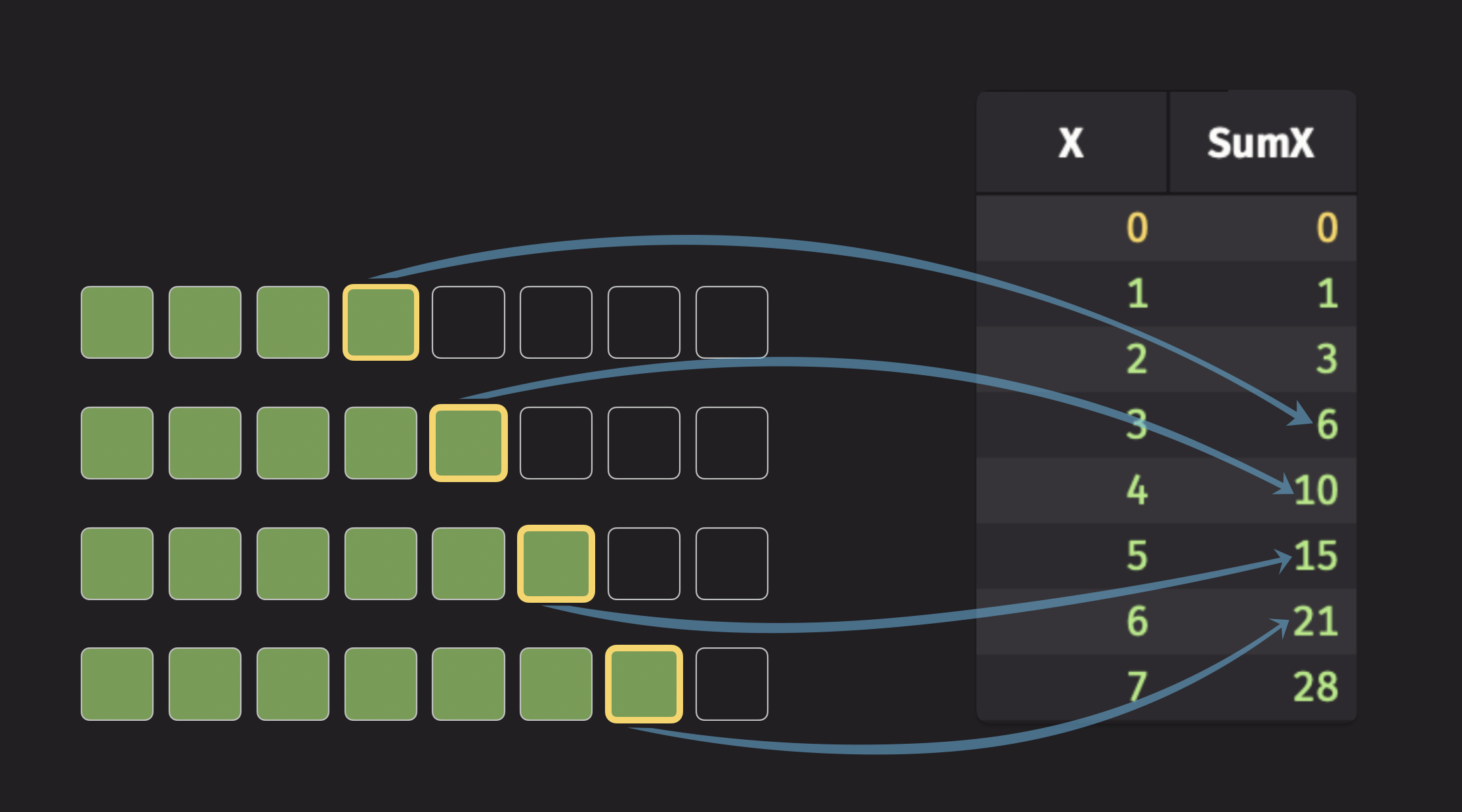
The code for the illustration above looks like this:

source = emptyTable(8).update("X = ii")

result = source.updateBy(CumSum("SumX=X"))

Cumulative average

The updateby module does not directly support a function to compute the cumulative average of a column. However, you can still compute the cumulative average by using two CumSum operations, where one of them is applied over a column of ones:

source = emptyTable(8).update("X = ii")

result = (
    source.update("Ones = 1")
    .updateBy(CumSum("SumX=X", "Ones"))
    .update("CumAvgX = SumX / Ones")
    .dropColumns("SumX", "Ones")
)

This demonstrates the flexibility of the updateBy table operation. If a particular kind of calculation is unavailable, it's almost always possible to accomplish with Deephaven.

Windowed aggregations

Windowed aggregations are similar to cumulative aggregations but operate on a finite-sized window of data. This means they only consider a limited number of rows for their calculations. The window size can be defined either by a number of rows (ticks) or by a duration of time.

Tick-based vs time-based windows

Tick-based windows aggregate values over a specified number of rows with fixed window sizes defined by revTicks and fwdTicks parameters:

• revTicks = 1, fwdTicks = 0 - Contains only the current row.
• revTicks = 10, fwdTicks = 0 - Contains 9 previous rows and the current row.
• revTicks = 0, fwdTicks = 10 - Contains the following 10 rows; excludes the current row.
• revTicks = 10, fwdTicks = 10 - Contains the previous 9 rows, the current row and the 10 rows following.
• revTicks = 10, fwdTicks = -5 - Contains 5 rows, beginning at 9 rows before, ending at 5 rows before the current row (inclusive).
• revTicks = 11, fwdTicks = -1 - Contains 10 rows, beginning at 10 rows before, ending at 1 row before the current row (inclusive).
• revTicks = -5, fwdTicks = 10 - Contains 5 rows, beginning 5 rows following, ending at 10 rows following the current row (inclusive).

Time-based windows aggregate values over time durations with variable window sizes defined by revTime and fwdTime parameters:

• revTime = "PT00:00:00", fwdTime = "PT00:00:00" - Contains rows that exactly match the current timestamp.
• revTime = "PT00:10:00", fwdTime = "PT00:00:00" - Contains rows from 10m earlier through the current timestamp (inclusive).
• revTime = "PT00:00:00", fwdTime = "PT00:10:00" - Contains rows from the current timestamp through 10m following the current row timestamp (inclusive).
• revTime = int(60e9), fwdTime = int(60e9) - Contains rows from 1m earlier through 1m following the current timestamp (inclusive).
• revTime = "PT00:10:00", fwdTime = "-PT00:05:00" - Contains rows from 10m earlier through 5m before the current timestamp (inclusive). This is a purely backward-looking window.
• revTime = int(-5e9), fwdTime = int(10e9) - Contains rows from 5s following through 10s following the current timestamp (inclusive). This is a purely forward-looking window.

Cumulative operators like CumSum are special cases of tick-based operators, where the window begins at the first table row and continues through to the current row.

Simple moving (rolling) aggregations

Simple moving (or rolling) aggregations are statistics computed over a finite, moving window of data. These operations weigh each data point in the window equally, regardless of its distance from the current row. The following simple moving statistics are supported:

Additional rolling operations

Deephaven offers two additional rolling operations that are not simple statistics, but rather for grouping or custom formulas:

The grouping operations collect values within the rolling window into an array. The custom formula operations allow you to define a custom formula that is applied to the values in the window.

To illustrate a simple moving aggregation, consider the rolling average. For each row, this operation calculates the average of all values within a specified window. The following illustration shows this:

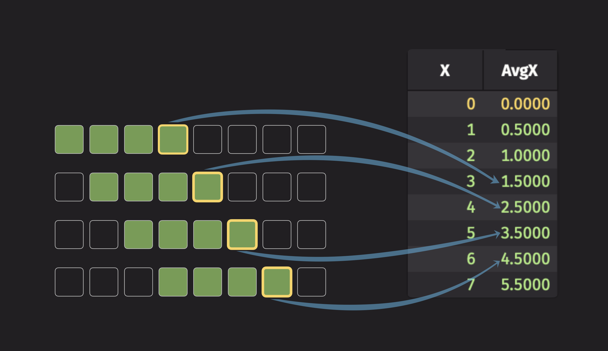
The code for the illustration above looks like this:

source = emptyTable(8).update("X = ii")

result = source.updateBy(RollingAvg(4, "AvgX=X"))

The following example demonstrates a series of different tick-based windows that look backwards, forwards, and both. Each example calculates the rolling sum of the Value column:

source = emptyTable(50).update("Value = ii")

updateByOps = [
    RollingSum(10, 0, "SumValueBackwards=Value"),
    RollingSum(1, 9, "SumValueForwards=Value"),
    RollingSum(6, 5, "SumValueBoth=Value"),
]

result = source.updateBy(updateByOps)

The above example can be modified to use time-based windows instead of tick-based windows:

source = emptyTable(50).update(
    "Timestamp = '2025-05-01T09:30:00 ET' + ii * SECOND",
    "Value = ii"
)

updateByOps = [
    RollingSum("Timestamp", parseDuration("PT10s"), parseDuration("PT00:00:00"), "SumValueBackwards=Value"),
    RollingSum("Timestamp", parseDuration("PT00:00:00"), parseDuration("PT10s"), "SumValueForwards=Value"),
    RollingSum("Timestamp", parseDuration("PT5s"), parseDuration("PT5s"), "SumValueBoth=Value"),
]

result = source.updateBy(updateByOps)

Rolling average

When creating a tick-based rolling operation, the revTicks parameter can configure how far the window extends behind the row. The current row is considered to belong to the backward-looking window, so setting revTicks=10 includes the current row and previous 9 rows.

The following example creates 2, 3, and 5-row backward-looking tick-based simple moving averages. These averages are computed by group, as specified with the by argument:

source = emptyTable(10).update("Letter = (i % 2 == 0) ? `A` : `B`", "X = randomInt(0, 100)")

sma2 = RollingAvg(2, "AvgX2=X")
sma3 = RollingAvg(3, "AvgX3=X")
sma5 = RollingAvg(5, "AvgX5=X")

result = source.updateBy([sma2, sma3, sma5], "Letter")

Here's another example that creates 3, 5, and 9-row windows, centered on the current row:

source = emptyTable(10).update("Letter = (i % 2 == 0) ? `A` : `B`", "X = randomInt(0, 100)")

// using fwdTicks gives windows that extend into the future
sma3 = RollingAvg(2, 1, "AvgX2=X")
sma5 = RollingAvg(3, 2, "AvgX3=X")
sma9 = RollingAvg(5, 4, "AvgX5=X")

result = source.updateBy([sma3, sma5, sma9], "Letter")

Time-based rolling average

Time-based rolling operations use a syntax similar to tick-based operations but require a timestamp column to be specified. This example uses the RollingAvg function to compute 2-second, 3-second, and 5-second moving averages:

source = emptyTable(10).update(
        "Timestamp = '2023-01-01T00:00:00 ET' + i * SECOND",
        "Letter = (i % 2 == 0) ? `A` : `B`",
        "X = randomInt(0, 25)",
)

sma2sec = RollingAvg("Timestamp", parseDuration("PT00:00:02"), "AvgX2Sec=X")
sma3sec = RollingAvg("Timestamp", parseDuration("PT3s"), "AvgX3Sec=X")
sma5sec = RollingAvg("Timestamp", parseDuration("PT3s"), "AvgX5Sec=X")

result = source.updateBy([sma2sec, sma3sec, sma5sec], "Letter")

Like before, you can use fwdTime to create windows into the future. Here's an example that creates 2-second, 5-second, and 10-second windows, centered on the current row:

source = emptyTable(10).update(
        "Timestamp = '2023-01-01T00:00:00 ET' + i * SECOND",
        "Letter = (i % 2 == 0) ? `A` : `B`",
        "X = randomInt(0, 25)",
)

sma2sec = RollingAvg("Timestamp", parseDuration("PT00:00:01"), parseDuration("PT00:00:01"), "AvgX2Sec=X")
sma5sec = RollingAvg("Timestamp", parseDuration("PT2.5s"), parseDuration("PT2.5s"), "AvgX3Sec=X")
sma10sec = RollingAvg("Timestamp", parseDuration("PT5s"), parseDuration("PT5s"), "AvgX5Sec=X")

result = source.updateBy([sma2sec, sma5sec, sma10sec], "Letter")

Exponential moving aggregations

Exponential moving statistics are another form of moving aggregations. Unlike simple moving aggregations that use a fixed window, these statistics use all preceding data points. However, they assign more weight to recent data and exponentially down-weight older data. This means distant observations have little effect on the result, while closer observations have a greater influence. The rate at which the weight decreases is controlled by a decay parameter. The following exponential moving statistics are supported:

To visualize an exponential moving statistic, consider the exponential moving average (EMA). The following illustration shows this:

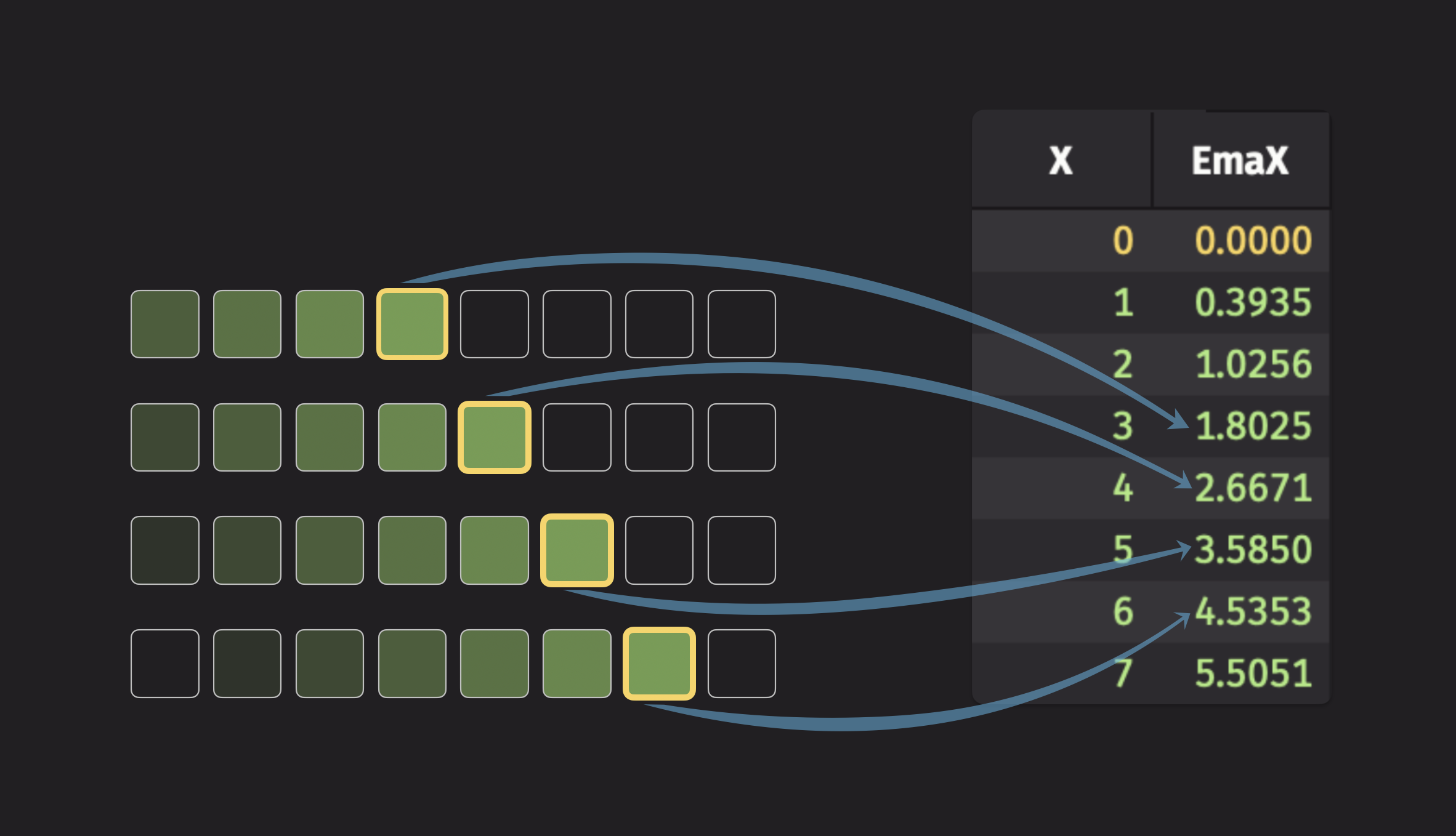
The code for the illustration above looks like this:

source = emptyTable(8).update("X = ii")

result = source.updateBy(Ema(2, "EmaX=X"))

The following example demonstrates the effect that different decay rates have on the exponential moving average:

source = emptyTable(10).update("Letter = (i % 2 == 0) ? `A` : `B`", "X = randomInt(0, 100)")

ema2 = Ema(2, "EMAX2=X")
ema3 = Ema(3, "EMAX3=X")
ema5 = Ema(5, "EMAX5=X")

result = source.updateBy([ema2, ema3, ema5], "Letter")

Understanding decay parameters

Tick-based decay (decayTicks):

• Smaller values = faster decay, more weight on recent data.
• decayTicks=1: Each previous row has ~37% the weight of the current row.
• decayTicks=10: Each previous row has ~90% the weight of the current row.
• Higher values create smoother, slower-responding averages.

Time-based decay (decayTime):

• Controls how quickly older data loses influence over time.
• decayTime="PT1s": Data from 1 second ago has ~37% weight.
• decayTime="PT10s": Data from 10 seconds ago has ~37% weight.
• Longer decay times create more stable, less responsive averages.

The same example can be modified to use time-based windows instead of tick-based windows:

source = emptyTable(50).update(
        "Timestamp = '2023-01-01T00:00:00 ET' + i * SECOND",
        "Letter = (i % 2 == 0) ? `A` : `B`",
        "X = randomInt(0, 25)",
)

ema2sec = Ema("Timestamp", parseDuration("PT2s"), "EmaX2Sec=X")
ema3sec = Ema("Timestamp", parseDuration("PT00:00:03"), "EmaX3=X")
ema5sec = Ema("Timestamp", parseDuration("PT5s"), "EmaX5=X",)

result = source.updateBy([ema2sec, ema3sec, ema5sec], "Letter")

In this time-based example:

• decayTime="PT2s": Creates a fast-responding average where data loses ~63% influence after 2 seconds.
• decayTime="PT4s": Medium responsiveness, data loses ~63% influence after 4 seconds.
• decayTime="PT6s": Slower response, data loses ~63% influence after 6 seconds.

Bollinger Bands

Bollinger bands are an application of moving statistics frequently used in financial applications.

To compute Bollinger Bands:

1. Compute the moving average.
2. Compute the moving standard deviation.
3. Compute the upper and lower envelopes.

Tick-based Bollinger Bands using simple moving statistics

When computing tick-based Bollinger bands, updateBy, RollingAvg and RollingStd are used to compute the average and envelope. Here, revTicks is the moving average decay rate in ticks and is used to specify the size of the rolling window.

// Generate some random example data

source = emptyTable(1000).update(
        "Timestamp='2023-01-13T12:00 ET' + i*MINUTE",
        "Ticker = i%2==0 ? `ABC` : `XYZ`",
        "Price = i%2==0 ? 100*sin(i/40)+100*random() : 100*cos(i/40)+100*random()+i/2",
)

// Compute the Bollinger Bands

revTicks = 20

// Coverage parameter - determines the width of the bands
w = 2

result = source.updateBy(
    [
        RollingAvg(revTicks, "AvgPrice=Price"),
        RollingAvg(revTicks, "StdPrice=Price"),
    ],
    "Ticker",
).update("Upper = AvgPrice + w*StdPrice", "Lower = AvgPrice - w*StdPrice")

// Plot the Bollinger Bands

def plotBollinger = { t, ticker ->
    d = t.where("Ticker=`${ticker}`")
    plot = plot("Price", d, "Timestamp", "Price")
        .plot("AvgPrice", d, "Timestamp", "AvgPrice")
        .plot("Upper", d, "Timestamp", "Upper")
        .plot("Lower", d, "Timestamp", "Lower")
        .show()
    return d
}


fAbc = plotBollinger(result, "ABC")
fXyz = plotBollinger(result, "XYZ")

Time-based Bollinger Bands using simple moving statistics

When computing time-based Bollinger Bands, updateBy, RollingAvg and RollingStd are used to compute the average and envelope. Here, revTime is the moving average window time.

// Generate some random example data

source = emptyTable(1000).update(
        "Timestamp='2023-01-13T12:00 ET' + i*MINUTE",
        "Ticker = i%2==0 ? `ABC` : `XYZ`",
        "Price = i%2==0 ? 100*sin(i/40)+100*random() : 100*cos(i/40)+100*random()+i/2"
)

// Compute the Bollinger Bands

revTime = "PT00:20:00"
// Coverage parameter - determines the width of the bands
w = 2

result = source.updateBy(
    [
        RollingAvg("Timestamp", parseDuration(revTime), "AvgPrice=Price"),
        RollingStd("Timestamp", parseDuration(revTime), "StdPrice=Price"),
    ],
    "Ticker",
).update("Upper = AvgPrice + w*StdPrice", "Lower = AvgPrice - w*StdPrice")

// Plot the Bollinger Bands

def plotBollinger = { t, ticker ->
    d = t.where("Ticker=`${ticker}`")
    plot = plot("Price", d, "Timestamp", "Price")
        .plot("AvgPrice", d, "Timestamp", "AvgPrice")
        .plot("Upper", d, "Timestamp", "Upper")
        .plot("Lower", d, "Timestamp", "Lower")
        .show()
    return d
}

fAbc = plotBollinger(result, "ABC")
fXyz = plotBollinger(result, "XYZ")

Tick-based Bollinger Bands using exponential moving statistics

When computing tick-based Bollinger Bands, updateBy, Ema and EmStd are used to compute the average and envelope. Here, decayTicks is the moving average decay rate in ticks and is used to specify the weighting of previous data points.

// Generate some random example data

source = emptyTable(1000).update(
        "Timestamp='2023-01-13T12:00 ET' + i*MINUTE",
        "Ticker = i%2==0 ? `ABC` : `XYZ`",
        "Price = i%2==0 ? 100*sin(i/40)+100*random() : 100*cos(i/40)+100*random()+i/2"
)

// Compute the Bollinger Bands

decayTicks = 20
// Coverage parameter - determines the width of the bands
w = 2

result = source.updateBy(
    [
        Ema(decayTicks, "EmaPrice=Price"),
        EmStd(decayTicks, "StdPrice=Price"),
    ],
    "Ticker",
).update("Upper = EmaPrice + w*StdPrice", "Lower = EmaPrice - w*StdPrice")

// Plot the Bollinger Bands

def plotBollinger = { t, ticker ->
    d = t.where("Ticker=`${ticker}`")
    plot = plot("Price", d, "Timestamp", "Price")
        .plot("AvgPrice", d, "Timestamp", "EmaPrice")
        .plot("Upper", d, "Timestamp", "Upper")
        .plot("Lower", d, "Timestamp", "Lower")
        .show()
    return d
}

fAbc = plotBollinger(result, "ABC")
fXyz = plotBollinger(result, "XYZ")

Time-based Bollinger Bands using exponential moving statistics

When computing time-based Bollinger Bands, updateBy, Ema and EmStd are used to compute the average and envelope. Here, decayTime is the moving average decay rate in time and is used to specify the weighting of new data points.

// Generate some random example data

source = emptyTable(1000).update(
        "Timestamp='2023-01-13T12:00 ET' + i*MINUTE",
        "Ticker = i%2==0 ? `ABC` : `XYZ`",
        "Price = i%2==0 ? 100*sin(i/40)+100*random() : 100*cos(i/40)+100*random()+i/2",
)

// Compute the Bollinger Bands

decayTime = "PT00:20:00"

// Coverage parameter - determines the width of the bands
w = 2

result = source.updateBy(
    [
        Ema("Timestamp", parseDuration(decayTime), "EmaPrice=Price"),
        Ema("Timestamp", parseDuration(decayTime), "StdPrice=Price"),
    ],
    "Ticker",
).update("Upper = EmaPrice + w*StdPrice", "Lower = EmaPrice - w*StdPrice")

// Plot the Bollinger Bands

def plotBollinger = { t, ticker ->
    d = t.where("Ticker=`${ticker}`")
    plot = plot("Price", d, "Timestamp", "Price")
        .plot("AvgPrice", d, "Timestamp", "EmaPrice")
        .plot("Upper", d, "Timestamp", "Upper")
        .plot("Lower", d, "Timestamp", "Lower")
        .show()
    return d
}



fAbc = plotBollinger(result, "ABC")
fXyz = plotBollinger(result, "XYZ")

Rolling formulas

The updateBy module enables users to create custom rolling aggregations with the RollingFormula function.

The user-defined formula can utilize any of Deephaven's built-in functions, arithmetic operators, or even user-defined Groovy functions.

Tick-based rolling formulas

Use RollingFormula to create custom tick-based rolling formulas. Here's an example that computes the rolling geometric mean of a column X by group:

source = emptyTable(100).update("Letter = (i % 2 == 0) ? `A` : `B`", "X = randomInt(0, 100)")

result = source.updateBy(
    RollingFormula(3, "pow(product(x), 1/count(x))", "x", "GeomMeanX=X"), "Letter"
)

Time-based rolling formulas

RollingFormula can also be used to create custom time-based rolling formulas. You must supply a timestamp column, and can specify the time window as backward-looking, forward-looking, or both. Here's an example that computes the 5-second rolling geometric mean of a column X by group:

source = emptyTable(100).update(
        "Timestamp = '2023-01-01T00:00:00 ET' + i * SECOND",
        "Letter = (i % 2 == 0) ? `A` : `B`",
        "X = randomInt(0, 25)",
)

result = source.updateBy(
    RollingFormula("Timestamp", 5_000_000, "pow(product(x), 1/count(x))", "x", "GeomMeanX=X"),
    "Letter"
)

Rolling groups

In addition to custom rolling formulas, updateby provides the ability to create rolling groups with RollingGroup. The grouped data are represented as arrays. See the guide on how to work with arrays for more details.

Tick-based rolling groups

Use RollingGroup to create tick-based rolling groups, where each group will have a specified number of entries determined by revTicks and fwdTicks. Here's an example that creates rolling groups with the three previous rows and the current row:

source = emptyTable(100).update("Letter = randomBool() ? `A` : `B`", "X = randomInt(0, 100)")

result = source.updateBy(RollingGroup(4, "GroupX=X"), "Letter")

To create groups that include data after the current row, use the fwdTicks parameter. This example creates a group that consists of the two previous rows, the current row, and the next four rows:

source = emptyTable(100).update("Letter = randomBool() ? `A` : `B`", "X = randomInt(0, 100)")

result = source.updateBy(RollingGroup(3, 4, "GroupX=X"), "Letter")

Time-based rolling groups

Similarly, use RollingGroup to create time-based rolling groups:

source = emptyTable(100).update(
        "Timestamp = '2023-01-01T00:00:00 ET' + i * SECOND",
        "Letter = randomBool() ? `A` : `B`",
        "X = randomInt(0, 25)",
)

result = source.updateBy(
    RollingGroup("Timestamp", parseDuration("PT3s"), "GroupX=X"),
    "Letter",
)

These groups are timestamp-based, so they are not guaranteed to contain elements from any previous row. This is in contrast to tick-based RollingGroup, which always yields groups of a fixed size after that size has been reached.

The fwdTime parameter is used to create groups that include rows occuring after the current row. Here's an example that creates rolling groups out of every row within five seconds of the current row:

source = emptyTable(100).update(
        "Timestamp = '2023-01-01T00:00:00 ET' + i * SECOND",
        "Letter = randomBool() ? `A` : `B`",
        "X = randomInt(0, 25)",
)

result = source.updateBy(RollingGroup("Timestamp", parseDuration("PT5s"), parseDuration("PT5s"), "GroupX=X"), "Letter")

Additional operations

updateBy also supports several other operations that are not strictly rolling aggregations. This section provides a brief overview of these operations with examples.

Sequential difference

The Delta operation calculates the difference between a row's value and the previous row's value in a given column. This is useful for calculating the rate of change. The following example demonstrates this:

source = emptyTable(100).update(
    "Timestamp = '2023-01-01T00:00:00 ET' + i * SECOND",
    "X = randomInt(0, 25)",
)

result = source.updateBy(Delta("DiffX=X"))

Sequential differences can be calculated on a per-group basis like all other updateBy operations. The following example demonstrates this:

source = emptyTable(100).update(
        "Timestamp = '2023-01-01T00:00:00 ET' + i * SECOND",
        "Letter = randomBool() ? `A` : `B`",
        "X = randomInt(0, 25)",
)

result = source.updateBy(Delta("DiffX=X"), "Letter")

Detrend time-series data

Sequential differencing is often used as a first measure for detrending time-series data. The updateby module provides the Delta function to make this easy:

source = emptyTable(1000).update(
    "Timestamp='2023-01-13T12:00 ET' + i*MINUTE",
    "Ticker = i%2==0 ? `ABC` : `XYZ`",
    "Price = i%2==0 ? 100*sin(i/40)+100*random() : 100*cos(i/40)+100*random()+i/2",
)

result = source.updateBy(Delta("DiffPrice=Price"), "Ticker")

noDetrend = plot("ABC", result.where("Ticker = `ABC`"), "Timestamp", "Price")
    .plot("XYZ", result.where("Ticker = `XYZ`"), "Timestamp", "Price")
    .show()

detrend = plot("ABC", result.where("Ticker = `ABC`"), "Timestamp", "DiffPrice")
    .plot("XYZ", result.where("Ticker = `XYZ`"), "Timestamp", "DiffPrice")
    .show()

Null handling

The Delta function takes an optional deltaControl argument to determine how null values are treated. You must supply a DeltaControl instance to use this argument. The following behaviors are available:

• DeltaControl.NULL_DOMINATES: A valid value following a null value returns null.
• DeltaControl.VALUE_DOMINATES: A valid value following a null value returns the valid value.
• DeltaControl.ZERO_DOMINATES: A valid value following a null value returns zero.

source = emptyTable(100).update(
    "Timestamp = '2023-01-01T00:00:00 ET' + i * SECOND",
    "Letter = randomBool() ? `A` : `B`",
    "X = randomInt(0, 25)",
)

result = source.updateBy(
    [
        Delta("DefaultDeltaX=X"),
        Delta(DeltaControl.NULL_DOMINATES, "NullDomDeltaX=X"),
        Delta(DeltaControl.VALUE_DOMINATES, "ValueDomDeltaX=X"),
        Delta(DeltaControl.ZERO_DOMINATES, "ZeroDomDeltaX=X"),
    ],
    "Letter",
)

By default, Delta uses NULL_DOMINATES, so differencing a number from a null will always return a null.

Forward fill

The Fill operation fills in null values with the most recent non-null value. This is useful for filling in missing data points in a time series. The following example demonstrates this:

source = emptyTable(100).update(
        "Timestamp = '2023-01-01T00:00:00 ET' + i * SECOND",
        "Letter = randomBool() ? `A` : `B`",
        "X = randomBool() ? NULL_INT : randomInt(0, 25)",
)

result = source.updateBy(Fill("FillX=X"), "Letter")

Choose the right aggregation

Choosing the right aggregation method depends on your specific use case and data requirements. Consider these key questions:

aggBy vs updateBy

aggBy and updateBy share some distinct similarities and differences. Understanding how the two relate to each other is important for understanding when to use each of them.

aggBy is functionally equivalent to sumBy, avgBy, minBy, etc. When you see sumBy in examples below, know that you could replace it with aggBy(AggSum(cols), by=groups) to achieve the same result. Both approaches perform the same aggregation operations.

Similarities

Both operations perform aggregations on a table. For instance, you can calculate a cumulative sum with both. Additionally, both operations also support performing aggregations over groups of rows, such as calculating the average price of a given stock, or the sum of sales for a given product.

Differences

There are two main differences between the two operations:

aggBy output

The output table of a single aggregation or multiple aggregation only contains one row for each group. To illustrate this, consider the following example, which calculates the aggregated sum of the Value column for each ID in the source table:

source = emptyTable(100).update("ID = randomInt(0, 4)", "Value = randomDouble(0, 1)")

result = source.sumBy("ID")

If the input table is ticking, then the value in each row of the output table changes when the input table ticks.

updateBy output

updateBy produces an output table that contains the same number of rows as the input table. Each row in the output table contains the aggregated value up to that point for the corresponding group. This means that updateBy keeps data history while performing the aggregation. To illustrate this, the previous example is modified to use updateBy instead of sumBy:

source = emptyTable(100).update("ID = randomInt(0, 4)", "Value = randomDouble(0, 1)")

result = source.updateBy(CumSum("Value"), "ID")

Note how the result table has the same number of rows as the source table. You can look back at previous values to see what the aggregated value was at any point in the table's history.

Use aggBy (or sumBy, avgBy, etc.) when you want a single aggregated result per group. The output contains one row for each group with the final aggregated value.

Use updateBy when you need to see the progression of aggregated values over time. The output preserves all rows from the source table, showing how the aggregation evolves.

Do you need to preserve data history?

• Use aggBy (or sumBy, avgBy, etc.) when you want a single aggregated result per group. The output contains one row for each group with the final aggregated value.
• Use updateBy when you need to see the progression of aggregated values over time. The output preserves all rows from the source table, showing how the aggregation evolves.

Capturing data history with traditional aggregations

While updateBy naturally preserves data history, it's also possible to capture some data history with traditional single aggregations and multiple aggregations. However, this requires a key column that places rows into buckets, such as intervals of time.

For example, you can create time-based buckets to see how aggregations change over different time periods:

source = emptyTable(10).update(
    "TimeGroup = i / 5",
    "Symbol = i % 2 == 0 ? `A` : `B`",
    "Volume = i + 1"
)

result = source.sumBy("TimeGroup", "Symbol")

In this example, the traditional aggregation groups data into buckets (using TimeGroup to simulate time intervals), showing how aggregated values change across different groups while providing partial history.

For more information on splitting temporal data into buckets of time, see Downsampling.

What type of aggregation window do you need?

• Cumulative aggregations (CumSum, CumMax, etc.): Use when you want to aggregate all data from the beginning up to the current row.
• Windowed aggregations: Use when you only want to consider a subset of recent data:
  • Tick-based windows (RollingSum, etc.): Use when your window should be defined by a fixed number of rows.
  • Time-based windows (RollingSum with timestamp, etc.): Use when your window should be defined by a time duration and you have a timestamp column.

How should recent vs. distant data be weighted?

• Simple moving aggregations (RollingAvg, RollingSum, etc.): Use when all data points in the window should be weighted equally.
• Exponential moving aggregations (Ema, EmMax, etc.): Use when recent data should have more influence than older data, with exponential decay over time.

Do you need custom calculations?

• Standard operations: Use built-in functions like RollingSum, RollingAvg, CumMax, etc. for common statistical calculations.
• Custom formulas: Use RollingFormula when you need to apply custom mathematical expressions to windowed data.
• Grouping operations: Use RollingGroup when you need to collect data into arrays for further processing.

Do you need to handle missing or erroneous data?

• Forward fill: Use Fill to replace null values with the most recent non-null value.
• Sequential differences: Use Delta to calculate row-to-row changes, useful for detrending time-series data.
• Error handling: Some operations like Ema support OperationControl parameters for handling null, NaN, or other erroneous values.

Performance considerations

• Rolling aggregations are more performant than rolling groups followed by calculations.
• Tick-based operations maintain separate windows per group, while time-based operations use timestamps across the entire table.
• Exponential moving aggregations use all historical data but weight recent observations more heavily.

Handling erroneous data

It's common for tables to contain null, NaN, or other erroneous values. Different updateBy operations handle these values in various ways:

Operations with explicit error handling controls

Certain operations can be configured to handle erroneous data through control parameters:

• Ema: Use control parameter with OperationControl.
• Delta: Use deltaControl parameter with DeltaControl.

Default null handling behavior

Most updateBy operations have consistent default behavior for null values:

• Cumulative operations (CumSum, CumMax, etc.): Skip null values and continue with the last valid result.
• Rolling operations (RollingAvg, RollingSum, etc.): Exclude null values from window calculations.
• Exponential operations (Ema, EmMax, etc.): Skip null values unless configured otherwise via OperationControl.

Specialized null handling operations

• Fill: Specifically designed to replace null values with the most recent non-null value.
• Delta: Configurable null handling through DeltaControl (see Null handling section).

For detailed configuration options, see the OperationControl reference guide.

Related documentation

• Create an empty table
• Create a time table
• Dedicated aggregations
• Combined aggregations
• Downsampling
• Select, view, and update
• Handle nulls, infs, and NaNs
• How to create XY series plots
• How to work with arrays
• Formulas
• updateBy
• aggBy
• RollingFormula
• RollingGroup
• Delta
• Fill