Cumulative, rolling, and moving statistics with update_by

This guide explains how to use Deephaven's update_by table operation and the updateby Python module to add cumulative, rolling, and moving statistics to a table.

update_by vs updateby

This document refers to update_by and updateby throughout. They are not identical:

• update_by always refers to theupdate_by table operation. This is always invoked as a method on a table:

result = source.update_by(...)

• updateby refers to the Python module housing all of the functions, like updateby.rolling_avg_time, that could be passed to update_by. This module is imported as uby in this guide:

import deephaven.updateby as uby

result = source.update_by(uby.rolling_avg_time(...))

This distinction will be important to keep in mind as you progress through the document.

Cumulative statistics

Cumulative statistics are the simplest operations in the updateby Python module. They are ordinary statistics computed over all previous data. The following cumulative statistics are currently supported in updateby:

Cumulative statistic	updateby function
Minimum	cum_min
Maximum	cum_max
Sum	cum_sum
Product	cum_prod

Cumulative sum

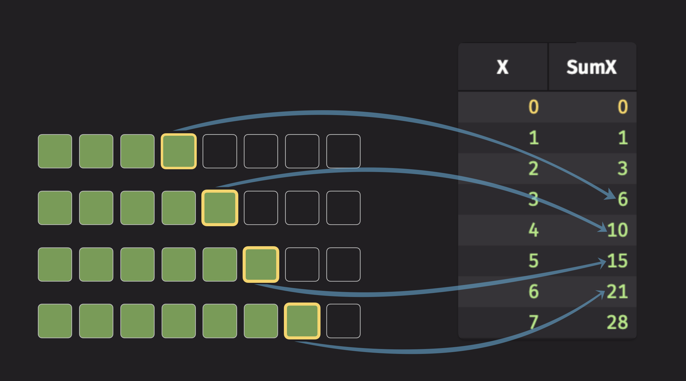
To illustrate a cumulative statistic, consider the cumulative sum. This operation computes the sum of all previous data points for every row in a table. Here's an illustration of the cumulative sum:

The fourth element of the cumulative sum column is the sum of the first four data points, the fifth element is the sum of the first five data points, and so on.

This calculation is implemented in Deephaven with the cum_sum function and the update_by table operation:

from deephaven import empty_table
import deephaven.updateby as uby

source = empty_table(8).update("X = ii")

result = source.update_by(uby.cum_sum("SumX=X"))

result

Here, the "SumX=X" argument indicates that the resulting column will be renamed SumX.

Cumulative average

The updateby module does not directly support a function to compute the cumulative average of a column. However, you can still compute the cumulative average by using two cum_sum operations, where one of them is applied over a column of ones:

from deephaven import empty_table
import deephaven.updateby as uby

source = empty_table(8).update("X = ii")

result = (
    source.update("Ones = 1")
    .update_by(uby.cum_sum(["SumX=X", "Ones"]))
    .update("CumAvgX = SumX / Ones")
    .drop_columns(["SumX", "Ones"])
)

result

This demonstrates the flexibility of the update_by table operation. If a particular kind of calculation is unavailable, it's almost always possible to accomplish with Deephaven.

Time-based vs tick-based operations

updateby functions use a window of data that is measured either by ticks (number of rows) or by specifying a time window. When using tick-based operators, the window is fixed in size and contains the data elements within the specified number of rows relative to the current row. Ticks can be specified as backward ticks (rev_ticks), forward ticks (fwd_ticks), or both. Here are some examples:

• rev_ticks = 1, fwd_ticks = 0 - Contains only the current row.
• rev_ticks = 10, fwd_ticks = 0 - Contains 9 previous rows and the current row.
• rev_ticks = 0, fwd_ticks = 10 - Contains the following 10 rows; excludes the current row.
• rev_ticks = 10, fwd_ticks = 10 - Contains the previous 9 rows, the current row and the 10 rows following.
• rev_ticks = 10, fwd_ticks = -5 - Contains 5 rows, beginning at 9 rows before, ending at 5 rows before the current row (inclusive).
• rev_ticks = 11, fwd_ticks = -1 - Contains 10 rows, beginning at 10 rows before, ending at 1 row before the current row (inclusive).
• rev_ticks = -5, fwd_ticks = 10 - Contains 5 rows, beginning 5 rows following, ending at 10 rows following the current row (inclusive).

For time-based operators, a timestamp column must be specified. The window will contain the data elements within the specified time period of the current row's timestamp. The number of rows in a time-based window will not be fixed and may actually be empty depending on the sparsity of the data. Time can be specified in terms of backward-looking time (rev_time), forward-looking time (fwd_time), or both. Here are some examples:

• rev_time = "PT00:00:00", fwd_time = "PT00:00:00" - Contains rows that exactly match the current timestamp.
• rev_time = "PT00:10:00", fwd_time = "PT00:00:00" - Contains rows from 10m earlier through the current timestamp (inclusive).
• rev_time = "PT00:00:00", fwd_time = "PT00:10:00" - Contains rows from the current timestamp through 10m following the current row timestamp (inclusive).
• rev_time = int(60e9), fwd_time = int(60e9) - Contains rows from 1m earlier through 1m following the current timestamp (inclusive).
• rev_time = "PT00:10:00", fwd_time = "-PT00:05:00" - Contains rows from 10m earlier through 5m before the current timestamp (inclusive). This is a purely backward-looking window.
• rev_time = int(-5e9), fwd_time = int(10e9) - Contains rows from 5s following through 10s following the current timestamp (inclusive). This is a purely forward-looking window.

Cumulative operators like cum_sum are special cases of tick-based operators, where the window begins at the first table row and continues through to the current row.

Simple moving (rolling) statistics

Simple moving (or rolling) statistics are ordinary statistics computed over a moving data window. Here are the simple moving statistics that Deephaven supports and the updateby functions that implement them:

Simple moving statistic	Tick-based	Time-based
Count	rolling_count_tick	rolling_count_time
Minimum	rolling_min_tick	rolling_min_time
Maximum	rolling_max_tick	rolling_max_time
Sum	rolling_sum_tick	rolling_sum_time
Product	rolling_prod_tick	rolling_prod_time
Average	rolling_avg_tick	rolling_avg_time
Weighted Average	rolling_wavg_tick	rolling_wavg_time
Standard Deviation	rolling_std_tick	rolling_std_time

Deephaven also offers the rolling_group_tick and rolling_group_time functions for creating rolling groups, and the rolling_formula_tick and rolling_formula_time for implementing custom rolling operations using DQL.

Tick-based rolling average

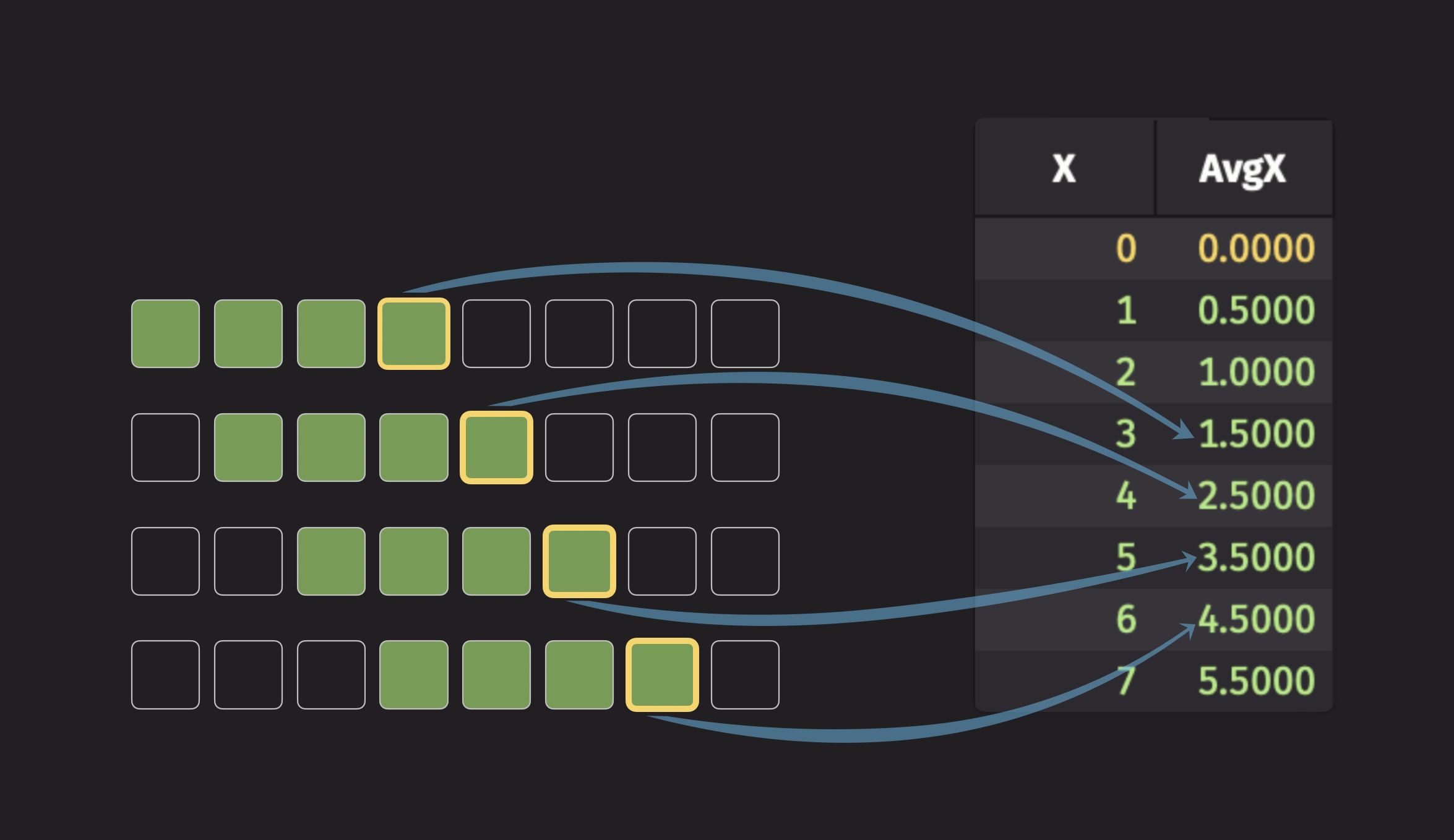
To illustrate a simple moving statistic, consider the simple moving average. It is the average of all data points inside of a given window, and that window moves across the dataset to generate the simple moving average for each row. Here is an illustration of a 4-tick moving average:

The fourth element of the moving average column is the average of the first four data points, the fifth element is the average of the second through fifth data points, and so on.

This calculation is implemented in Deephaven using the rolling_avg_tick function and the update_by table operation:

from deephaven import empty_table
import deephaven.updateby as uby

source = empty_table(8).update("X = ii")

result = source.update_by(uby.rolling_avg_tick("AvgX=X", rev_ticks=4))

result

When creating a tick-based rolling operation, the rev_ticks parameter can configure how far the window extends behind the row. The current row is considered to belong to the backward-looking window, so setting rev_ticks=10 includes the current row and previous 9 rows.

The following example creates 2, 3, and 5-row backward-looking tick-based simple moving averages. These averages are computed by group, as specified with the by argument:

from deephaven import empty_table
import deephaven.updateby as uby

source = empty_table(10).update(
    ["Letter = (i % 2 == 0) ? `A` : `B`", "X = randomInt(0, 100)"]
)

sma_2 = uby.rolling_avg_tick(cols=["AvgX2=X"], rev_ticks=2)
sma_3 = uby.rolling_avg_tick(cols=["AvgX3=X"], rev_ticks=3)
sma_5 = uby.rolling_avg_tick(cols=["AvgX5=X"], rev_ticks=5)

result = source.update_by(ops=[sma_2, sma_3, sma_5], by="Letter")

result

Here's another example that creates 3, 5, and 9-row windows, centered on the current row:

from deephaven import empty_table
import deephaven.updateby as uby

source = empty_table(10).update(
    ["Letter = (i % 2 == 0) ? `A` : `B`", "X = randomInt(0, 100)"]
)

# using fwd_ticks gives windows that extend into the future
sma_3 = uby.rolling_avg_tick(cols=["AvgX2=X"], rev_ticks=2, fwd_ticks=1)
sma_5 = uby.rolling_avg_tick(cols=["AvgX3=X"], rev_ticks=3, fwd_ticks=2)
sma_9 = uby.rolling_avg_tick(cols=["AvgX5=X"], rev_ticks=5, fwd_ticks=4)

result = source.update_by(ops=[sma_3, sma_5, sma_9], by="Letter")

result

Time-based rolling average

Time-based rolling operations use a syntax similar to tick-based operations but require a timestamp column to be specified. This example uses the rolling_avg_time function to compute 2-second, 3-second, and 5-second moving averages:

from deephaven import empty_table
import deephaven.updateby as uby

source = empty_table(10).update(
    [
        "Timestamp = '2023-01-01T00:00:00 ET' + i * SECOND",
        "Letter = (i % 2 == 0) ? `A` : `B`",
        "X = randomInt(0, 25)",
    ]
)

sma_2_sec = uby.rolling_avg_time(
    ts_col="Timestamp", cols="AvgX2Sec=X", rev_time="PT00:00:02"
)
sma_3_sec = uby.rolling_avg_time(ts_col="Timestamp", cols="AvgX3Sec=X", rev_time="PT3s")
sma_5_sec = uby.rolling_avg_time(ts_col="Timestamp", cols="AvgX5Sec=X", rev_time="PT5s")

result = source.update_by(ops=[sma_2_sec, sma_3_sec, sma_5_sec], by="Letter")

result

Like before, you can use fwd_time to create windows into the future. Here's an example that creates 2-second, 5-second, and 10-second windows, centered on the current row:

from deephaven import empty_table
import deephaven.updateby as uby

source = empty_table(10).update(
    [
        "Timestamp = '2023-01-01T00:00:00 ET' + i * SECOND",
        "Letter = (i % 2 == 0) ? `A` : `B`",
        "X = randomInt(0, 25)",
    ]
)

sma_2_sec = uby.rolling_avg_time(
    ts_col="Timestamp", cols="AvgX2Sec=X", rev_time="PT00:00:01", fwd_time="PT00:00:01"
)
sma_5_sec = uby.rolling_avg_time(
    ts_col="Timestamp", cols="AvgX3Sec=X", rev_time="PT2.5s", fwd_time="PT2.5s"
)
sma_10_sec = uby.rolling_avg_time(
    ts_col="Timestamp", cols="AvgX5Sec=X", rev_time="PT5s", fwd_time="PT5s"
)

result = source.update_by(ops=[sma_2_sec, sma_5_sec, sma_10_sec], by="Letter")

result

Exponential moving statistics

Exponential moving statistics are another form of moving statistics that depart from the concept of a sliding window of data. Instead, these statistics utilize all of the data that comes before a given data point, as cumulative statistics do. However, they place more weight on recent data points and down-weight distant ones. This means that distant observations have little effect on the moving statistic, while closer observations carry more weight. The larger the decay_rate parameter is, the more weight distant observations carry. Here are the exponential moving statistics that Deephaven supports and the updateby functions that implement them:

Exponential moving statistic	Tick-based	Time-based
Minimum (EMMin)	emmin_tick	emmin_time
Maximum (EMMax)	emmax_tick	emmax_time
Sum (EMS)	ems_tick	ems_time
Average (EMA)	ema_tick	ema_time
Standard Deviation (EMStd)	emstd_tick	emstd_time

Tick-based exponential moving average

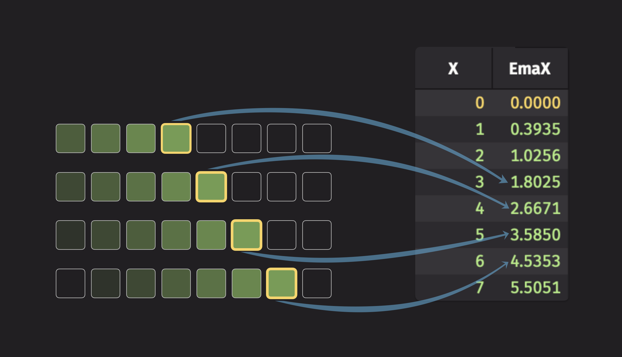
To illustrate an exponential moving statistic, consider the exponential moving average (EMA). Here's a visualization of the EMA:

Each element in the new column depends on every data point that came before it, but distant data points only have a very small effect. Check out the reference documentation for ema_tick for the formula used to compute this statistic.

This calculation is implemented in Deephaven using the ema_tick function and the update_by table operation:

from deephaven import empty_table
import deephaven.updateby as uby

source = empty_table(8).update("X = ii")

result = source.update_by(uby.ema_tick(decay_ticks=2, cols="EmaX=X"))

result

The following example shows how to create exponential moving averages with decay rates of 2, 3, and 5. These averages are computed by group, as specified with the by argument:

from deephaven import empty_table
import deephaven.updateby as uby

source = empty_table(10).update(
    ["Letter = (i % 2 == 0) ? `A` : `B`", "X = randomInt(0, 100)"]
)

ema_2 = uby.ema_tick(decay_ticks=2, cols="EMAX2=X")
ema_3 = uby.ema_tick(decay_ticks=3, cols="EMAX3=X")
ema_5 = uby.ema_tick(decay_ticks=5, cols="EMAX5=X")

result = source.update_by(ops=[ema_2, ema_3, ema_5], by="Letter")

result

Time-based exponential moving average

Time-based exponential moving statistics are conceptually similar to tick-based exponential moving statistics but measure the distance between observations in terms of time rather than the number of rows between them. Check out the reference documentation for ema_time for the formula used to compute this statistic.

Here is an example similar to the time-based simple moving average that utilizes the EMA with decay times of 2 seconds, 3 seconds, and 5 seconds:

from deephaven import empty_table
import deephaven.updateby as uby

source = empty_table(50).update(
    [
        "Timestamp = '2023-01-01T00:00:00 ET' + i * SECOND",
        "Letter = (i % 2 == 0) ? `A` : `B`",
        "X = randomInt(0, 25)",
    ]
)

ema_2_sec = uby.ema_time(ts_col="Timestamp", decay_time="PT2s", cols="EmaX2Sec=X")
ema_3_sec = uby.ema_time(ts_col="Timestamp", decay_time="PT00:00:03", cols="EmaX3=X")
ema_5_sec = uby.ema_time(ts_col="Timestamp", decay_time="PT5s", cols="EmaX5=X")

result = source.update_by(ops=[ema_2_sec, ema_3_sec, ema_5_sec], by="Letter")

result

Bollinger Bands

Bollinger bands are an application of moving statistics frequently used in financial applications.

To compute Bollinger Bands:

1. Compute the moving average.
2. Compute the moving standard deviation.
3. Compute the upper and lower envelopes.

Tick-based Bollinger Bands using simple moving statistics

When computing tick-based Bollinger bands, update_by, rolling_avg_tick and rolling_std_tick are used to compute the average and envelope. Here, rev_ticks is the moving average decay rate in ticks and is used to specify the size of the rolling window.

from deephaven import empty_table
import deephaven.updateby as uby
from deephaven.plot import Figure

# Generate some random example data

source = empty_table(1000).update(
    [
        "Timestamp='2023-01-13T12:00 ET' + i*MINUTE",
        "Ticker = i%2==0 ? `ABC` : `XYZ`",
        "Price = i%2==0 ? 100*sin(i/40)+100*random() : 100*cos(i/40)+100*random()+i/2",
    ]
)

# Compute the Bollinger Bands

rev_ticks = 20
# Coverage parameter - determines the width of the bands
w = 2

result = source.update_by(
    [
        uby.rolling_avg_tick("AvgPrice=Price", rev_ticks=rev_ticks),
        uby.rolling_std_tick("StdPrice=Price", rev_ticks=rev_ticks),
    ],
    by="Ticker",
).update(["Upper = AvgPrice + w*StdPrice", "Lower = AvgPrice - w*StdPrice"])

# Plot the Bollinger Bands


def plot_bollinger(t, ticker):
    d = t.where(f"Ticker=`{ticker}`")

    return (
        Figure()
        .plot_xy(series_name="Price", t=d, x="Timestamp", y="Price")
        .plot_xy(series_name="AvgPrice", t=d, x="Timestamp", y="AvgPrice")
        .plot_xy(series_name="Upper", t=d, x="Timestamp", y="Upper")
        .plot_xy(series_name="Lower", t=d, x="Timestamp", y="Lower")
        .show()
    )


f_abc = plot_bollinger(result, "ABC")
f_xyz = plot_bollinger(result, "XYZ")

f_abc

f_xyz

source

result

Time-based Bollinger Bands using simple moving statistics

When computing time-based Bollinger Bands, update_by, rolling_avg_time and rolling_std_time are used to compute the average and envelope. Here, rev_time is the moving average window time.

from deephaven import empty_table
import deephaven.updateby as uby
from deephaven.plot import Figure

# Generate some random example data

source = empty_table(1000).update(
    [
        "Timestamp='2023-01-13T12:00 ET' + i*MINUTE",
        "Ticker = i%2==0 ? `ABC` : `XYZ`",
        "Price = i%2==0 ? 100*sin(i/40)+100*random() : 100*cos(i/40)+100*random()+i/2",
    ]
)

# Compute the Bollinger Bands

rev_time = "PT00:20:00"
# Coverage parameter - determines the width of the bands
w = 2

result = source.update_by(
    [
        uby.rolling_avg_time("Timestamp", "AvgPrice=Price", rev_time=rev_time),
        uby.rolling_std_time("Timestamp", "StdPrice=Price", rev_time=rev_time),
    ],
    by="Ticker",
).update(["Upper = AvgPrice + w*StdPrice", "Lower = AvgPrice - w*StdPrice"])

# Plot the Bollinger Bands


def plot_bollinger(t, ticker):
    d = t.where(f"Ticker=`{ticker}`")

    return (
        Figure()
        .plot_xy(series_name="Price", t=d, x="Timestamp", y="Price")
        .plot_xy(series_name="AvgPrice", t=d, x="Timestamp", y="AvgPrice")
        .plot_xy(series_name="Upper", t=d, x="Timestamp", y="Upper")
        .plot_xy(series_name="Lower", t=d, x="Timestamp", y="Lower")
        .show()
    )


f_abc = plot_bollinger(result, "ABC")
f_xyz = plot_bollinger(result, "XYZ")

f_abc

f_xyz

source

result

Tick-based Bollinger Bands using exponential moving statistics

When computing tick-based Bollinger Bands, update_by, ema_tick and emstd_tick are used to compute the average and envelope. Here, decay_ticks is the moving average decay rate in ticks and is used to specify the weighting of previous data points.

from deephaven import empty_table
import deephaven.updateby as uby
from deephaven.plot import Figure

# Generate some random example data

source = empty_table(1000).update(
    [
        "Timestamp='2023-01-13T12:00 ET' + i*MINUTE",
        "Ticker = i%2==0 ? `ABC` : `XYZ`",
        "Price = i%2==0 ? 100*sin(i/40)+100*random() : 100*cos(i/40)+100*random()+i/2",
    ]
)

# Compute the Bollinger Bands

decay_ticks = 20
# Coverage parameter - determines the width of the bands
w = 2

result = source.update_by(
    [
        uby.ema_tick(decay_ticks=decay_ticks, cols="EmaPrice=Price"),
        uby.emstd_tick(decay_ticks=decay_ticks, cols="StdPrice=Price"),
    ],
    by=["Ticker"],
).update(["Upper = EmaPrice + w*StdPrice", "Lower = EmaPrice - w*StdPrice"])

# Plot the Bollinger Bands


def plot_bollinger(t, ticker):
    d = t.where(f"Ticker=`{ticker}`")

    return (
        Figure()
        .plot_xy(series_name="Price", t=d, x="Timestamp", y="Price")
        .plot_xy(series_name="EmaPrice", t=d, x="Timestamp", y="EmaPrice")
        .plot_xy(series_name="Upper", t=d, x="Timestamp", y="Upper")
        .plot_xy(series_name="Lower", t=d, x="Timestamp", y="Lower")
        .show()
    )


f_abc = plot_bollinger(result, "ABC")
f_xyz = plot_bollinger(result, "XYZ")

f_abc

f_xyz

source

result

Time-based Bollinger Bands using exponential moving statistics

When computing time-based Bollinger Bands, update_by, ema_time and emstd_time are used to compute the average and envelope. Here, decay_time is the moving average decay rate in time and is used to specify the weighting of new data points.

from deephaven import empty_table
import deephaven.updateby as uby
from deephaven.plot import Figure

# Generate some random example data

source = empty_table(1000).update(
    [
        "Timestamp='2023-01-13T12:00 ET' + i*MINUTE",
        "Ticker = i%2==0 ? `ABC` : `XYZ`",
        "Price = i%2==0 ? 100*sin(i/40)+100*random() : 100*cos(i/40)+100*random()+i/2",
    ]
)

# Compute the Bollinger Bands

decay_time = "PT00:20:00"
# Coverage parameter - determines the width of the bands
w = 2

result = source.update_by(
    [
        uby.ema_time("Timestamp", decay_time=decay_time, cols="EmaPrice=Price"),
        uby.emstd_time("Timestamp", decay_time=decay_time, cols="StdPrice=Price"),
    ],
    by=["Ticker"],
).update(["Upper = EmaPrice + w*StdPrice", "Lower = EmaPrice - w*StdPrice"])

# Plot the Bollinger Bands


def plot_bollinger(t, ticker):
    d = t.where(f"Ticker=`{ticker}`")

    return (
        Figure()
        .plot_xy(series_name="Price", t=d, x="Timestamp", y="Price")
        .plot_xy(series_name="EmaPrice", t=d, x="Timestamp", y="EmaPrice")
        .plot_xy(series_name="Upper", t=d, x="Timestamp", y="Upper")
        .plot_xy(series_name="Lower", t=d, x="Timestamp", y="Lower")
        .show()
    )


f_abc = plot_bollinger(result, "ABC")
f_xyz = plot_bollinger(result, "XYZ")

f_abc

f_xyz

source

result

Related documentation

• Create a time table
• Create an empty table
• How to create XY series plots
• How to use select, view, and update
• How to use update_by
• Handle nulls, infs, and NaNs
• ema_time
• ema_tick
• emstd_tick
• emstd_time
• Formulas
• User-Defined Functions